5.14 MCMC for DINA model in STAN
STAN is another very popular MCMC program and one can use rstan in R to run stan code. STAN uses different algorithms from JAGS and nimble. A limitation of STAN is that it cannot handle discrete variable directly.
Recall that in nimble and JAGS, one needs to specify the probability of obtaining a score for each student on each item, which serves as the likelihood.
In STAN, we have to marginalize the discrete variables.
Recall that the log likelihood of item response matrix \(\mathbf{Y}\) of all \(N\) students can be written by \[\begin{equation} \ell(\mathbf{Y}) = \log \prod\limits_{i = 1}^N L ({\mathbf{Y}_i}) = \sum\limits_{i = 1}^N \log L({\mathbf{Y}_i}) \end{equation}\] where the marginalized log likelihood observing a response vector \(\mathbf{Y}_i\) for student \(i\) is \[\begin{equation} \log L({\mathbf{Y}_i})=\log \sum_cL( {\mathbf{Y}_i}|{\alpha_i=\alpha_c})p(\mathbf{\alpha}_c) \end{equation}\]
The code below, which was adopted from here, can be used.
Code
data{
  int<lower=1> J;         // # of items
  int<lower=1> N;         // # of respondents
  int<lower=1> K;         // # of attributes
  int<lower=1> C;         // # of attribute profiles (latent classes)
  matrix[N,J] y;          // response matrix
  matrix[C,J] eta;      // eta matrix
  matrix[J,K] Q;
}

parameters{
  simplex[C] pi;                   // probabilities of latent class membership
  real<lower=0,upper=1> s[J];      // slip parameter
  real<lower=0,upper=1> g[J];      // guess parameter
}

transformed parameters{
  vector[C] log_pi;
  log_pi = log(pi);
}

model{
  real ps[C];
  real pj;
  real log_items[J];
  s ~ beta(1,1);
  g ~ beta(1,1);
  for (i in 1:N){
    for (c in 1:C){
      for (j in 1:J){
        pj = g[j] + (1-s[j]-g[j])*eta[c,j];
        log_items[j] = y[i,j] * log(pj) + (1 - y[i,j]) * log(1 - pj);
      }
      ps[c] = log_pi[c] + sum(log_items);
    }
    target += log_sum_exp(ps);
  }
}
Code
library(GDINA)
score <- sim10GDINA$simdat
Q <- sim10GDINA$simQ
J <- ncol(score)
K=ncol(Q)
N=nrow(score)
all.patterns <- GDINA::attributepattern(K)
C <- nrow(all.patterns)

eta <- matrix(NA,C,J)
for(l in 1:C){
  for(j in 1:J){
    eta[l,j] <- 1 * (drop(all.patterns[l,]%*%Q[j,])>=sum(Q[j,]))
  }
}

dina_data <- list(N = N, J = J, K = K, C = C, y = score, eta = eta)


stan_inits <- list(list(g = runif(J, 0.1, 0.3), s = runif(J, 0.1, 0.3)),
                   list(g = runif(J, 0.2, 0.4), s = runif(J, 0.2, 0.4)))

# Fit model to simulated data
library(rstan)
dina_stan_mcmc <- stan(file = "dina.stan", data = dina_data,
                         chains = 2, iter = 5000,warmup =  2500, init = stan_inits)
Code
## mean sd 2.5% 50% 97.5% Rhat n.eff
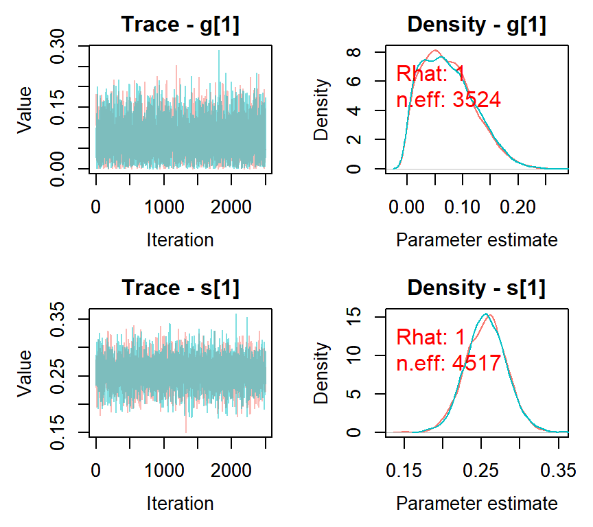
## s[1] 0.26 0.03 0.20 0.26 0.31 1 4517
## s[2] 0.28 0.03 0.22 0.28 0.33 1 5522
## s[3] 0.11 0.02 0.07 0.11 0.16 1 5857
## s[4] 0.20 0.03 0.14 0.20 0.25 1 4838
## s[5] 0.29 0.04 0.22 0.29 0.36 1 5319
## s[6] 0.07 0.02 0.04 0.07 0.11 1 6961
## s[7] 0.32 0.03 0.26 0.32 0.38 1 6037
## s[8] 0.30 0.04 0.23 0.30 0.37 1 3899
## s[9] 0.20 0.03 0.15 0.20 0.26 1 8282
## s[10] 0.16 0.03 0.10 0.16 0.22 1 6326
## g[1] 0.07 0.05 0.00 0.07 0.18 1 3524
## g[2] 0.09 0.03 0.04 0.09 0.16 1 4796
## g[3] 0.07 0.03 0.02 0.07 0.13 1 4278
## g[4] 0.22 0.02 0.18 0.22 0.27 1 6345
## g[5] 0.08 0.01 0.06 0.08 0.11 1 8461
## g[6] 0.59 0.03 0.53 0.59 0.64 1 5092
## g[7] 0.26 0.02 0.22 0.26 0.30 1 7905
## g[8] 0.15 0.02 0.11 0.15 0.19 1 6004
## g[9] 0.27 0.02 0.23 0.27 0.31 1 6979
## g[10] 0.34 0.02 0.30 0.33 0.37 1 6575Code