5.13 MCMC for DINA model in JAGS and R2jags R package

Zhan et al. (2019a) introduced how to use JAGS for Bayesian estimation for CDMs using MCMC algorithm. To use JAGS, you need to download and install GAGS from here.

The following code was adapted from Zhan et al. (2019a) and can be used for estimating parameters of the DINA model.

Code

#
Y <- sim10GDINA$simdat
Q <- sim10GDINA$simQ
all.patterns <- GDINA::attributepattern(ncol(Q))
jags.dina <- function() {
    for (n in 1:N) {
        for (i in 1:I) {
            eta[n, i] <- 1 * (sum(alpha[n, 1:K] * Q[i, 1:K]) >= sum(Q[i,
                1:K]))
            p[n, i] <- g[i] + (1 - s[i] - g[i]) * eta[n, i]
            Y[n, i] ~ dbern(p[n, i])
        }
        for (k in 1:K) {
            alpha[n, k] <- all.patterns[latent.group.index[n], k]
        }
        latent.group.index[n] ~ dcat(pi[1:C])
    }
    pi[1:C] ~ ddirch(delta[1:C])
    for (i in 1:I) {
        s[i] ~ dbeta(1, 1)
        g[i] ~ dbeta(1, 1) %_% T(0, 1 - s[i])
    }
}
library(R2jags)
N <- nrow(Y)
I <- nrow(Q)
K <- ncol(Q)
C <- nrow(all.patterns)
delta <- rep(1, C)
jags.data <- list("N", "I", "K", "Y", "Q", "C", "all.patterns", "delta")
jags.parameters <- c("s", "g", "latent.group.index", "pi")
jags.inits <- NULL
jags.dina.mcmc <- jags(data = jags.data, inits = jags.inits, parameters.to.save = jags.parameters,
    model.file = jags.dina, n.chains = 2, n.iter = 5000, n.burnin = 2500,
    n.thin = 1, DIC = TRUE)

Code

library(MCMCvis)
MCMCvis::MCMCsummary(jags.dina.mcmc, params = c('s','g'), 
            Rhat = TRUE,round = 2)

##       mean   sd 2.5%  50% 97.5% Rhat n.eff
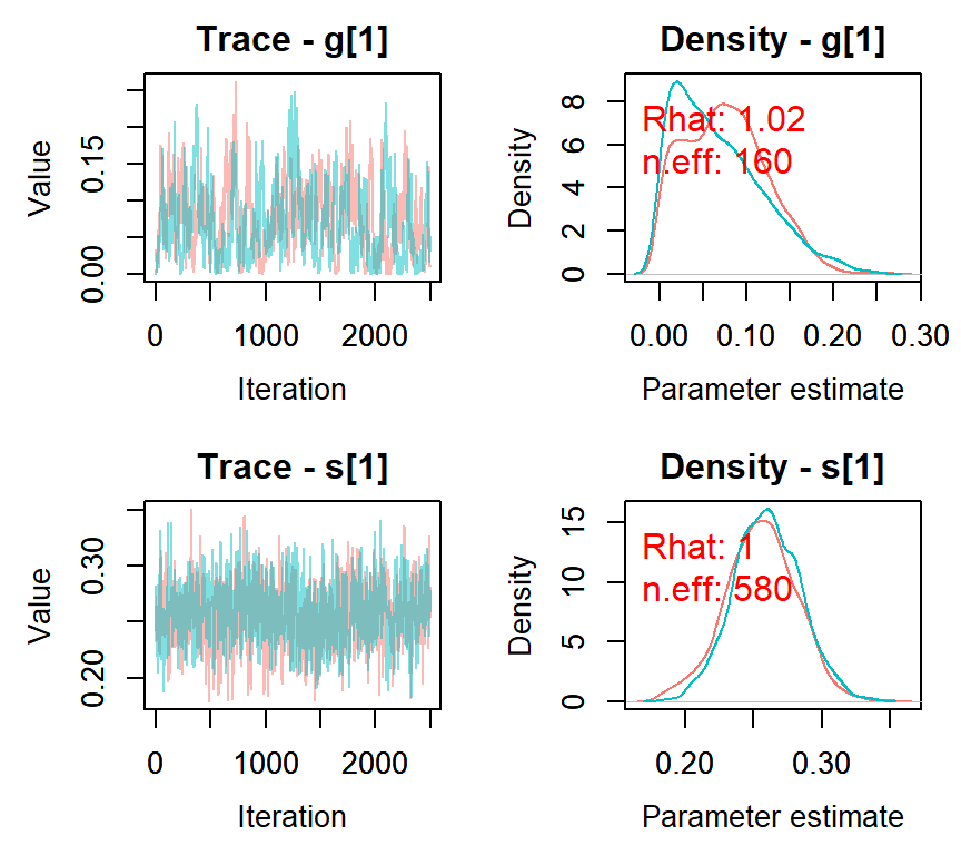
## s[1]  0.26 0.03 0.21 0.26  0.31    1   580
## s[2]  0.28 0.03 0.22 0.28  0.33    1   685
## s[3]  0.11 0.02 0.07 0.11  0.16    1   614
## s[4]  0.20 0.03 0.14 0.20  0.26    1   569
## s[5]  0.29 0.04 0.22 0.29  0.36    1   754
## s[6]  0.07 0.02 0.04 0.07  0.11    1   835
## s[7]  0.32 0.03 0.27 0.32  0.38    1   957
## s[8]  0.30 0.04 0.23 0.31  0.38    1   423
## s[9]  0.21 0.03 0.15 0.21  0.26    1  1257
## s[10] 0.16 0.03 0.10 0.16  0.23    1  1011
## g[1]  0.07 0.05 0.00 0.07  0.18    1   160
## g[2]  0.09 0.03 0.03 0.09  0.15    1   308
## g[3]  0.07 0.03 0.02 0.07  0.13    1   335
## g[4]  0.22 0.02 0.18 0.22  0.26    1   836
## g[5]  0.08 0.01 0.06 0.08  0.11    1  1342
## g[6]  0.59 0.03 0.53 0.59  0.63    1   959
## g[7]  0.26 0.02 0.22 0.26  0.30    1  1401
## g[8]  0.15 0.02 0.11 0.15  0.19    1   964
## g[9]  0.27 0.02 0.23 0.27  0.31    1  1142
## g[10] 0.33 0.02 0.30 0.34  0.37    1  1098

Code

MCMCvis::MCMCtrace(jags.dina.mcmc,params = c("g[1]","s[1]"),ISB = FALSE,
           exact = TRUE,
           ind = TRUE,
           pdf = FALSE,
           Rhat = TRUE,
           n.eff = TRUE,
           iter = 5000)

References

Zhan, P., Jiao, H., Man, K., & Wang, L. (2019a). Using JAGS for bayesian cognitive diagnosis modeling: A tutorial. Journal of Educational and Behavioral Statistics, 44(4), 473–503. https://doi.org/10.3102/1076998619826040