4.5 DINA model estimation

To estimate the DINA model, call GDINA function again and specify the data and Q-matrix as the first two arguments.

Code

#Fit the data using the DINA model
fit2 <- GDINA(dat = data1, Q = Q1, model = "DINA", verbose = 0)

To print some general model estimation information, type fit2 in Rstudio console:

Code

fit2

## Call:
## GDINA(dat = data1, Q = Q1, model = "DINA", verbose = 0)
## 
## GDINA version 2.9.4 (2023-07-01) 
## ===============================================
## Data
## -----------------------------------------------
## # of individuals    groups    items         
##              837         1       15
## ===============================================
## Model
## -----------------------------------------------
## Fitted model(s)       = DINA 
## Attribute structure   = saturated 
## Attribute level       = Dichotomous 
## ===============================================
## Estimation
## -----------------------------------------------
## Number of iterations  = 111 
## 
## For the final iteration:
##   Max abs change in item success prob. = 0.0001 
##   Max abs change in mixing proportions = 0.0001 
##   Change in -2 log-likelihood          = 0.0005 
##   Converged?                           = TRUE 
## 
## Time used             = 0.2303 secs

To extract item parameters, we can use coef function, as in

Code

coef(fit2)

## $`Item 1`
## P(0) P(1) 
## 0.91 0.98 
## 
## $`Item 2`
##  P(0)  P(1) 
## 0.078 0.759 
## 
## $`Item 3`
## P(0) P(1) 
## 0.55 0.77 
## 
## $`Item 4`
## P(0) P(1) 
## 0.37 0.83 
## 
## $`Item 5`
## P(00) P(10) P(01) P(11) 
##  0.41  0.41  0.41  0.91 
## 
## $`Item 6`
## P(00) P(10) P(01) P(11) 
##   0.2   0.2   0.2   0.7 
## 
## $`Item 7`
## P(00) P(10) P(01) P(11) 
##  0.22  0.22  0.22  0.77 
## 
## $`Item 8`
## P(00) P(10) P(01) P(11) 
##  0.30  0.30  0.30  0.74 
## 
## $`Item 9`
## P(00) P(10) P(01) P(11) 
##  0.25  0.25  0.25  0.62 
## 
## $`Item 10`
## P(00) P(10) P(01) P(11) 
##  0.43  0.43  0.43  0.70 
## 
## $`Item 11`
## P(00) P(10) P(01) P(11) 
##  0.62  0.62  0.62  0.85 
## 
## $`Item 12`
## P(00) P(10) P(01) P(11) 
##  0.29  0.29  0.29  0.62 
## 
## $`Item 13`
## P(00) P(10) P(01) P(11) 
##  0.22  0.22  0.22  0.53 
## 
## $`Item 14`
## P(000) P(100) P(010) P(001) P(110) P(101) P(011) P(111) 
##   0.28   0.28   0.28   0.28   0.28   0.28   0.28   0.63 
## 
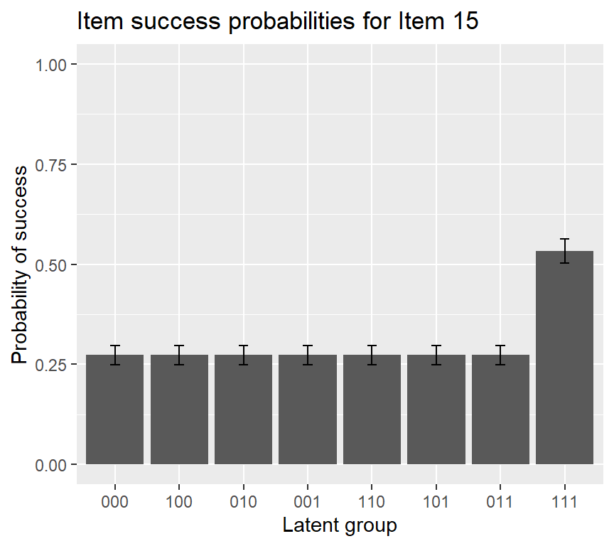
## $`Item 15`
## P(000) P(100) P(010) P(001) P(110) P(101) P(011) P(111) 
##   0.27   0.27   0.27   0.27   0.27   0.27   0.27   0.53

To obtain guessing and slip parameters, specify what = “gs”:

Code

coef(fit2, what = "gs")

##         guessing  slip
## Item 1     0.914 0.016
## Item 2     0.078 0.240
## Item 3     0.549 0.229
## Item 4     0.366 0.174
## Item 5     0.412 0.093
## Item 6     0.200 0.301
## Item 7     0.220 0.234
## Item 8     0.299 0.261
## Item 9     0.252 0.384
## Item 10    0.435 0.302
## Item 11    0.619 0.149
## Item 12    0.290 0.378
## Item 13    0.217 0.468
## Item 14    0.277 0.372
## Item 15    0.273 0.467

We can still draw the IRF plot of item 15, using the following code:

Code

plot(fit2, what = "IRF", item = c(15), withSE = TRUE)

To obtain attribute estimates, use the function personparm:

Code

head(personparm(fit2))

##      A1 A2 A3
## [1,]  1  1  1
## [2,]  0  0  1
## [3,]  1  1  0
## [4,]  0  1  0
## [5,]  0  0  0
## [6,]  1  1  1