8.2 Item-level Absolute Fit measures (Cont’d)

The code below shows how to calculate these item-level fit statistics in GDINA package:

Code

library(GDINA)
Y <- sim10GDINA$simdat
head(Y)

##      [,1] [,2] [,3] [,4] [,5] [,6] [,7] [,8] [,9] [,10]
## [1,]    1    0    1    1    0    1    1    1    0     1
## [2,]    1    1    1    1    1    1    1    1    0     1
## [3,]    1    1    1    0    1    1    1    0    1     0
## [4,]    1    0    1    1    1    1    1    1    1     0
## [5,]    0    0    1    1    0    0    1    0    0     0
## [6,]    1    0    0    0    0    0    0    1    0     1

Code

Q <- sim10GDINA$simQ
Q

##       [,1] [,2] [,3]
##  [1,]    1    0    0
##  [2,]    0    1    0
##  [3,]    0    0    1
##  [4,]    1    0    1
##  [5,]    0    1    1
##  [6,]    1    1    0
##  [7,]    1    0    1
##  [8,]    1    1    0
##  [9,]    0    1    1
## [10,]    1    1    1

We need to fit a model to the data first. Let us choose DINA model as an example.

Code

fit.dina <- GDINA(Y,Q,model = "DINA",verbose = 0)

We can then use itemfit() function to calculate item-level fit statistics:

Code

ift <- itemfit(fit.dina)

We can show the results of transformed correlation and log odds ratio using heatmap plot:

Code

plot(ift)

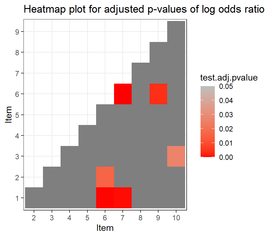
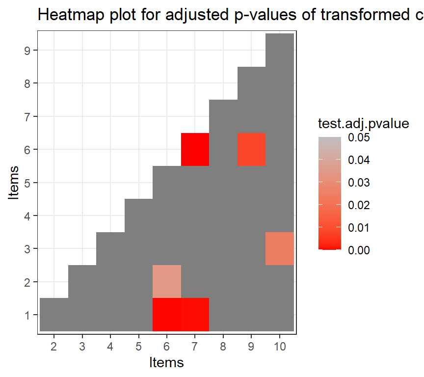
Note that transformed correlation and log odds ratio are at item-pair level. We can aggregate their results and report at item level.

Code

summary(ift)

## 
## Item-level fit statistics
##         z.prop pvalue[z.prop] max[z.r] pvalue.max[z.r] adj.pvalue.max[z.r] max[z.logOR] pvalue.max[z.logOR] adj.pvalue.max[z.logOR]
## Item 1   0.084           0.93      4.6          0.0000              0.0000          4.6              0.0000                  0.0000
## Item 2   0.051           0.96      3.3          0.0009              0.0077          3.5              0.0004                  0.0036
## Item 3   0.096           0.92      3.4          0.0006              0.0054          3.4              0.0007                  0.0060
## Item 4   0.052           0.96      2.2          0.0308              0.2768          2.2              0.0289                  0.2597
## Item 5   0.158           0.87      2.7          0.0070              0.0631          3.2              0.0016                  0.0140
## Item 6   0.257           0.80      5.3          0.0000              0.0000          5.5              0.0000                  0.0000
## Item 7   0.065           0.95      5.3          0.0000              0.0000          5.5              0.0000                  0.0000
## Item 8   0.040           0.97      3.0          0.0028              0.0249          3.0              0.0025                  0.0222
## Item 9   0.056           0.96      3.7          0.0002              0.0018          3.9              0.0001                  0.0009
## Item 10  0.086           0.93      3.4          0.0006              0.0054          3.4              0.0007                  0.0060

We can also aggregate the results and report at the test level:

Code

ift

## Summary of Item Fit Analysis
## 
## Call:
## itemfit(GDINA.obj = fit.dina)
## 
##                         mean[stats] max[stats] max[z.stats] p-value adj.p-value
## Proportion correct           0.0014     0.0036         0.26     0.8           1
## Transformed correlation      0.0517     0.1670         5.27     0.0           0
## Log odds ratio               0.2295     0.8124         5.55     0.0           0
## Note: p-value and adj.p-value are associated with max[z.stats].
##       adj.p-values are based on the holm method.