11.5 How to simulation data using a CDM

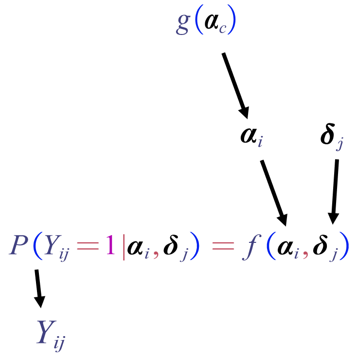
The diagram below shows how we generate the response of student \(i\) to item \(j\)

To generate a \(N\times J\) item response matrix, we need to repeat this process over all students and all items.

For illustration, let us consider one condition combination:

Code

N <- 100
K <- 5
J <- 15

In CDM, we need to have Q-matrix first:

Code

Q15 <- matrix(c(1, 0, 0, 0, 0, 0, 1, 0, 0, 0, 0, 0, 1, 0, 0, 0, 0, 0, 1,
    0, 0, 0, 0, 0, 1, 1, 1, 0, 0, 0, 0, 1, 1, 0, 0, 0, 0, 1, 1, 0, 0, 0,
    0, 1, 1, 1, 0, 0, 0, 1, 1, 1, 1, 0, 0, 0, 1, 1, 1, 0, 0, 0, 1, 1, 1,
    1, 0, 0, 1, 1, 1, 1, 0, 0, 1), ncol = K, nrow = J)

Huebner & Wang (2011) used the DINA model and generated slip and guess parameters randomly from the Uniform(.05, .30) and Uniform(.20, .45) distributions for the high and low diagnosticity settings, respectively (p.413). We only consider the low diagnosticity condition.

Code

# guessing and slip parameters
set.seed(12345)

gs <- matrix(runif(J * 2, 0.2, 0.45), ncol = 2)

Huebner & Wang (2011) also considered two distributions of attribute profiles. We will consider the so-called flat population for student population, which means all latent class sizes are equal, which is also referred to as a uniform distribution. In other words, all possible attribute profiles are equally likely to occur.

A sample can be simulated using simGDINA() function based on the above settings:

Code

set.seed(12345)
library(GDINA)
sim <- simGDINA(N = N, Q = Q15, gs.parm = gs, model = "DINA", att.dist = "uniform")

• To extract the simulated data or true attribute profiles, use extract() function. Specifically, to get the simulated data, specify what = dat:

Code

Y <- GDINA::extract(sim, what = "dat")
head(Y)

##      [,1] [,2] [,3] [,4] [,5] [,6] [,7] [,8] [,9] [,10] [,11] [,12] [,13] [,14] [,15]
## [1,]    0    0    1    1    1    0    0    0    0     1     1     1     1     0     0
## [2,]    0    0    0    1    0    1    0    0    1     0     0     0     0     0     0
## [3,]    0    1    0    1    0    1    0    0    0     1     0     0     1     0     0
## [4,]    0    1    1    1    0    0    0    1    1     0     0     0     0     0     1
## [5,]    0    0    1    1    0    0    1    0    1     0     1     0     0     0     0
## [6,]    0    0    1    1    0    0    0    1    1     1     1     0     0     0     1

• To extract the simulated (true) attribute profiles, specify what = “attribute”

Code

true.attributes <- GDINA::extract(sim, what = "attribute")
head(true.attributes)

##      A1 A2 A3 A4 A5
## [1,]  0  0  1  1  0
## [2,]  1  1  0  0  1
## [3,]  0  0  0  1  1
## [4,]  0  0  1  1  1
## [5,]  1  1  1  0  1
## [6,]  0  1  1  0  1

References

Huebner, A., & Wang, C. (2011). A note on comparing examinee classification methods for cognitive diagnosis models. Educational and Psychological Measurement, 71(2), 407–419.