Chapter 8 Practical. Introduction to jamovi
This chapter focuses on learning how to work with datasets in jamovi (The jamovi project, 2024). You can download jamovi (https://www.jamovi.org/) for free or run it directly from a browser using the jamovi cloud (https://www.jamovi.org/cloud.html). In this chapter, we will work with two datasets.
The first dataset includes some hypothetical measurements of soil organic carbon (grams of carbon per kilogram of soil) from topsoil and subsoil collected in a national park. Such data might be collected to understand how pyrogenic carbon (i.e., carbon produced by the charring of biomass during a fire) is stored in different landscape areas (Preston & Schmidt, 2006; Santín et al., 2016). These data can be downloaded online4.
The second dataset includes measurements of figs from trees of the Sonoran Desert Rock Fig (Ficus petiolaris) in Baja, Mexico (Figure 8.1). I collected these data in an effort to understand coexistence in a fig wasp community (Duthie et al., 2015; Duthie & Nason, 2016). Measurements include fig lengths, widths, and heights in centimetres from four different fig trees, and the number of seeds in each fruit. This dataset can also be downloaded online5.
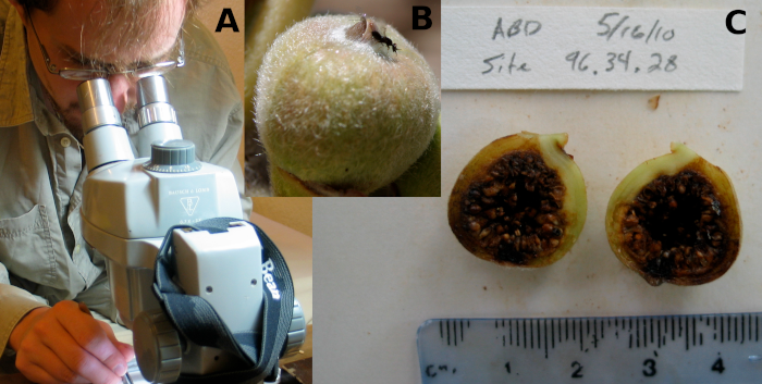
Figure 8.1: Three images showing the process of collecting data for the dimensions of figs from trees of the Sonoran Desert Rock Fig in Baja, Mexico. (A) Processing fig fruits, which included measuring the diameter of figs along three different axes of length, width, and height, (B) a fig still attached to a tree with a fig wasp on top of it, and (C) a sliced open fig with seeds along the inside of it.
This chapter will use the soil organic carbon dataset in Exercise 8.1 for summary statistics. The fig fruits dataset will be used for Exercise 8.2 on transforming variables and Exercise 8.3 on computing a variable. Some of these exercises will be similar to those of Chapter 3, but in jamovi rather than a separate spreadsheet.
8.1 Summary statistics
Once jamovi is open, you can import the soil organic carbon dataset by clicking on the three horizontal lines in the upper left corner of the tool bar, then selecting ‘Open’ (Figure 8.2).
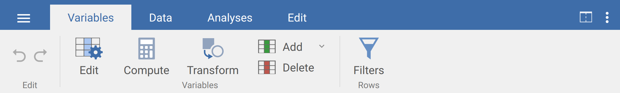
Figure 8.2: The jamovi toolbar including tabs for opening files, Variables, Data, Analyses, and Edit. To open a file, select the three horizontal lines in the upper left.
You might need to click ‘Browse’ in the upper right of jamovi to find the file. Once the data are imported, you should see two separate columns. The first column will show soil organic carbon values for topsoil samples, and the second column will show soil organic carbon values for subsoil samples. These data are not formatted in a tidy way. We need to fix this so that each row is a unique observation and each column is a variable (see Chapter 2). It might be easiest to reorganise the data in a spreadsheet such as LibreOffice Calc or Microsoft Excel. But you can also edit the data directly in jamovi by clicking on the ‘Data’ tab in the toolbar (Figures 8.3). The best way to reorganise the data in jamovi is to double-click on the third column of data next to ‘subsoil’ (see Figure 8.3).
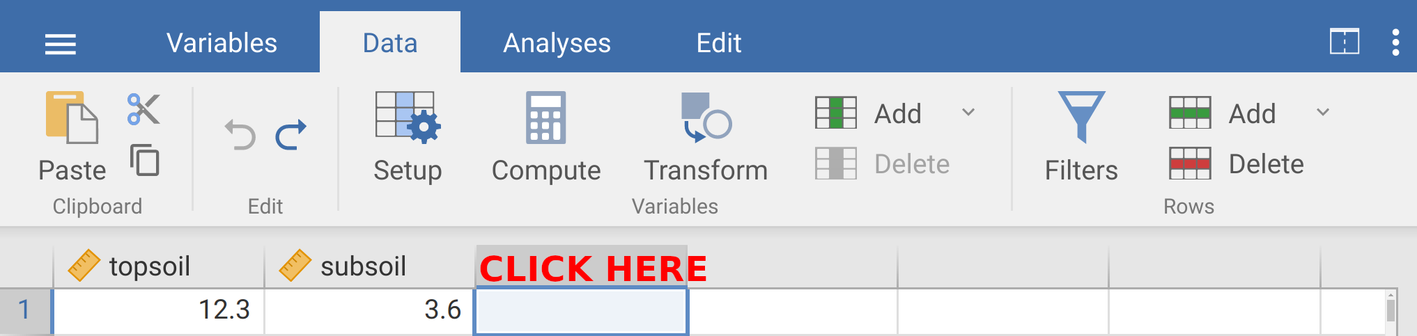
Figure 8.3: The jamovi toolbar is shown with the soil organic carbon dataset. In jamovi, double-clicking above column three where it says ‘CLICK HERE’ will allow you to input a new variable.
After double-clicking on the location shown in Figure 8.3, there will be three buttons visible.
You can click the ‘New Data Variable’ to insert a new variable named ‘soil_type’ in place of the default name ‘C’.
Keep the ‘Measure type’ as ‘Nominal’, but change the ‘Data type’ to ‘text’.
When you are done, click the > character to the right so that the variable is fixed (Figure 8.4).
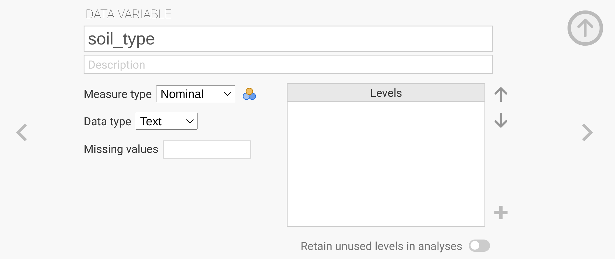
Figure 8.4: The jamovi toolbar is shown with the input for creating a new data variable. The new variable added is to indicate the soil type (topsoil or subsoil), so it needs to be a nominal variable with a data type of text.
After typing in the new variable ‘soil_type’, add another variable called ‘organic_carbon’. The organic_carbon variable should have a measure type of ‘Continuous’ and a data type of ‘Decimal’. After both soil_type and organic_carbon variables have been set, you can click the up arrow with the upper right circle (Figure 8.4) to get the new variable window out of the way.
With the two new variables created, we can now rearrange the data in a tidy format. The first 19 rows of soil_type should be ‘topsoil’, and the remaining 15 rows should be ‘subsoil’. To do this quickly, you can write ‘topsoil’ in the first row of soil_type and copy-paste into the remaining rows. You can do the same to write ‘subsoil’ in the remaining rows 20–34. Next, copy all of the topsoil values in column 1 into the first 19 rows of column 4, and copy all of the subsoil values in column 2 into the next 15 rows. After doing all of this, your column 3 (soil_type) should have the word ‘topsoil’ in rows 1–19 and ‘subsoil’ in rows 20–34. The values from columns 1 and 2 should now fill rows 1–34 of column 4. You can now delete the first column of data by right clicking on the column name ‘topsoil’ and selecting ‘Delete Variable’. Do the same for the second column ‘subsoil’. Now you should have a tidy dataset with two columns of data, one called ‘soil_type’ and one called ‘organic_carbon’. You are now ready to calculate some descriptive statistics from the data.
First, we can calculate the minimum, maximum, and mean of all of the organic carbon values (i.e., the ‘grand’ mean, which includes both soil types). To do this, select the ‘Analyses’ tab, then click on the left-most button called ‘Exploration’ in the toolbar.
After clicking on ‘Exploration’, a pull-down box will appear with an option for ‘Descriptives’. Select this option, and you will see a new window with our two columns of data in the left-most box. Click once on the ‘organic_carbon’ variable and use the right arrow to move it into the ‘Variables’ box. In the right-most panel of jamovi, a table called ‘Descriptives’ will appear, which will include values for the organic carbon mean, minimum, and maximum. Write these values on the lines below, and remember to include units.
Mean: ____________________________
Minimum: ____________________________
Maximum: ____________________________
These values might be useful, but recall that there are two different soil types that need to be considered: topsoil and subsoil. The mean, minimum, and maximum above pool both of these soil types together, but we might instead want to know the mean, minimum, and maximum values for topsoil and subsoil separately. Splitting organic carbon by soil type is straightforward in jamovi. To do it, go back to the Exploration \(\to\) Descriptives option and again put ‘organic_carbon’ in the Variables box. This time, however, notice the ‘Split by’ box below the Variables box. Now, click on ‘soil_type’ in the descriptives and click on the lower right arrow to move soil type into the ‘Split by’ box. The table of descriptives in the right window will now break down all of the summary statistics by soil type. First, write the mean, minimum, and maximum topsoil values below.
Topsoil mean: ____________________________
Topsoil minimum: ____________________________
Topsoil maximum: ____________________________
Next, do the same for the mean, minimum, and maximum subsoil values.
Subsoil mean: ____________________________
Subsoil minimum: ____________________________
Subsoil maximum: ____________________________
From the values above, the mean of organic carbon sampled from the topsoil appears to be greater than the mean of organic carbon sampled from the subsoil. Assuming that jamovi has calculated the means correctly, we can be confident that the topsoil sample mean is higher. But what about the population means? Think back to concepts of populations versus samples from Chapter 4. Based on these samples in the dataset, can we really say for certain that the population mean of topsoil is higher than the population mean of subsoil? Think about this, then write a sentence below about how confident we can be about concluding that topsoil organic carbon is greater than subsoil organic carbon.
What would make you more (or less) confident that topsoil and subsoil population means are different? Think about this, then write another sentence below that answers the question.
Note that there is no right or wrong answer for the above two questions. The entire point of the questions is to help you reflect on your own learning and better link the concepts of populations and samples to the real dataset in this practical. Doing this will make the statistical hypothesis testing that comes later in this book more clear.
8.2 Transforming variables
In this next exercise, we will work with the fig fruits dataset. Open this dataset into jamovi. Note that there are five columns of data, and all of the data appear to be in a tidy format. Each row represents a separate fig fruit, while each column represents a measured variable associated with the fruit. The first several rows should look like Table 8.1.
| Tree | Length_cm | Width_cm | Height_cm | Seeds |
|---|---|---|---|---|
| A | 1.5 | 1.8 | 1.4 | 238 |
| A | 1.7 | 1.9 | 1.5 | 198 |
| A | 2.1 | 2.1 | 1.6 | 220 |
| A | 1.5 | 1.6 | 1.4 | 188 |
| A | 1.6 | 1.6 | 1.5 | 139 |
| A | 1.5 | 1.4 | 1.5 | 173 |
The dataset includes the tree from which the fig was sampled in column 1 (A, B, C, and D), then the length, width, and height of the fig in centimetres. Finally, the last column shows how many seeds were counted within the fig. Use the Descriptives option in jamovi to find the grand (i.e., not split by Tree) mean length, width, and height of figs in the dataset. Write these means down below (remember the units).
Grand mean length: ____________________________
Grand mean height: ____________________________
Grand mean width: ____________________________
Now look at the different rows in the Descriptives table of jamovi. Note that there is a row for ‘Missing’, and there appears to be one missing value for fig width and fig height. This is very common in real datasets. Sometimes practical limitations in the field prevent data from being collected, or something happens that causes data to be lost. We therefore need to be able to work with datasets that have missing data. For now, we will just note the missing data and find them in the actual dataset. Go back to the ‘Data’ tab in jamovi and find the figs with a missing width and height value. Report the rows of these missing values below.
Missing width row: ____________________________
Missing height row: ____________________________
Next, we will go back to working with the actual data. Note that the length, width, and height variables are all recorded in centimetres to a single decimal place. Suppose we want to transform these variables so that they are represented in millimetres instead of centimetres We will start by creating a new column ‘Length_mm’ by transforming the existing ‘Length_cm’ column. To do this, click on the ‘Data’ tab at the top of the toolbar again, then click on the ‘Length_cm’ column name to highlight the entire column. Your screen should look like the image in Figure 8.5.
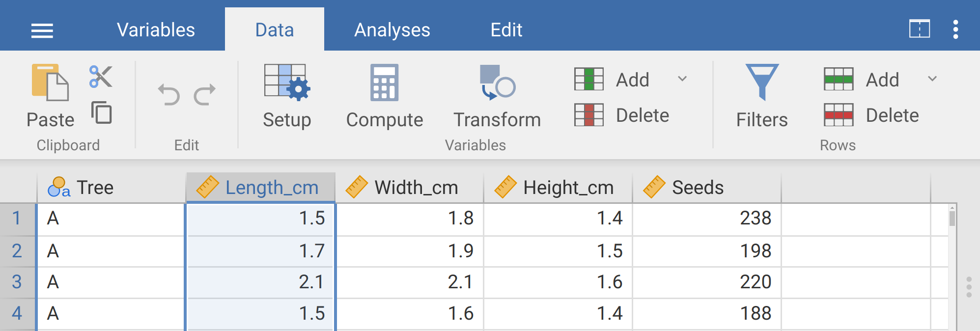
Figure 8.5: The jamovi toolbar where the tab ‘Data’ is selected. The length (cm) column is highlighted and will be transformed by clicking on the Transform button in the toolbar above.
With the ‘Length_cm’ column highlighted, click on the ‘Transform’ button in the toolbar.
Two things happen next.
First, a new column appears in the dataset that looks identical to ‘Length_cm’; ignore this for now.
Second, a box appears below the toolbar allowing us to type in a new name for the transformed variable.
We can call this variable ‘Length_mm’.
Below, note the first pull-down menu ‘Source variable’.
The source value should be ‘Length_cm’, so we can leave this alone.
The second pull-down menu ‘using transform’ will need to change.
To change the transform from ‘None’, click the arrow and select ‘Create New Transform’ from the pull-down.
A new box will pop up allowing us to name the transformation.
It does not matter what we call it (e.g., ‘cm_to_mm’ is fine).
Note that there are 10 mm in 1 cm, so to convert from centimetres to millimetres, we need to multiply the values of ‘Length_cm’ by 10.
We can do this by appending a ‘* 10’ to the lower box of the transform window, so that it reads ‘= $source * 10’ (Figure 8.6).
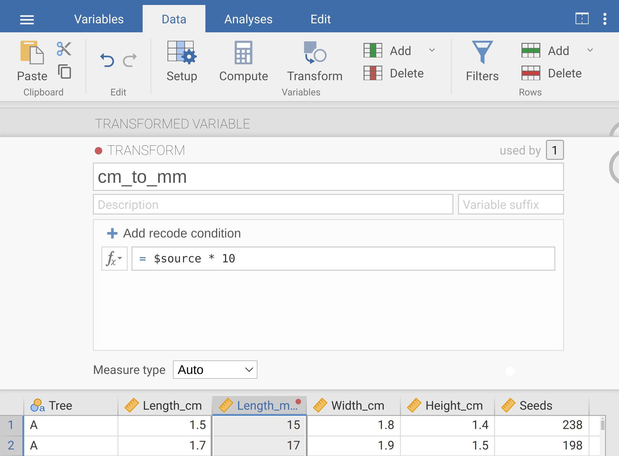
Figure 8.6: The jamovi toolbar where the tab ‘Data’ is selected. The box below shows the transform, which has been named ‘cm_to_mm’. The transformation occurs by multiplying the source (Length_mm) by 10. The dataset underneath shows the first few rows with the transformed column highlighted (note that the new ‘Length_mm’ column is 10 times the length column).
When we are finished, we can click the down arrow inside the circle in the upper right to get rid of the transform window, then the up arrow inside the circle in the upper right to get rid of the transformed variable window. Now we have a new column called ‘Length_mm’, in which values are 10 times greater than they are in the adjacent ‘Length_cm’ column, and therefore represent fig length in millimetres. If we want to, we can always change the transformation by double-clicking the ‘Length_mm’ column. For now, apply the same transformation to fig width and height, so we have three new columns of length, width, and height all measured in millimetres (note, if you want to, you can use the saved transformation ‘cm_to_mm’ that you used to transform length, saving some time). At the end of this, you should have eight columns of data, including three new columns that you just created by transforming the existing columns of Length_cm, Width_cm, and Height_cm into the new columns Length_mm, Width_mm, and Height_mm. Find the means of these three new columns and write them below.
Grand mean length (mm): ____________________________
Grand mean height (mm): ____________________________
Grand mean width (mm): ____________________________
Compare these means to the means calculated above in centimetres. Do the differences between means in centimetres and the means in millimetres make sense?
8.3 Computing variables
In this last exercise, we will compute a new variable ‘fig_volume’. Because of the way that the dimensions of the fig were measured in the field, we need to make some simplifying assumptions when calculating volume. We will assume that fig fruits are perfect spheres, and that the radius of each fig is half of its measured width (i.e., ‘Width_mm / 2’). This is obviously not ideal, but sometimes practical limitations in the field make it necessary to make these kinds of simplifying assumptions. In this case, how might assuming that figs are perfectly spherical affect the accuracy of our estimated fig volume? Write a sentence of reflection on this question below, drawing from what you learnt in Chapter 6 about accuracy and precision of measurements.
Now we are ready to make our calculation of fig volume. The formula for the volume of a sphere (\(V\)) given its radius \(r\) is,
\[V = \frac{4}{3} \pi r^{3}.\]
In words, sphere volume equals four-thirds times \(\pi\), times \(r\) cubed (i.e., \(r\) to the third power). If this equation is confusing, remember that \(\pi\) is approximately 3.14, and taking \(r\) to the third power means that we are multiplying \(r\) by itself 3 times. We could therefore rewrite the equation above,
\[V = \frac{4}{3} \times 3.14 \times r \times r \times r.\]
This is the formula that we can use to create our new column of data for fig volume. To do this, double-click on the first empty column of the dataset, just to the right of the ‘Seeds’ column header. You will see a pull-down menu in jamovi with three options, one of which is ‘NEW COMPUTED VARIABLE’. This is the option that we want. We need to name this new variable, so we can call it ‘fig_volume’. Next, we need to type in the formula for calculating volume. First, in the small box next to the \(f_{x}\), type in the (4/3) multiplied by 3.14 as below.
= (4/3) * 3.14Next, we need to multiply by the variable ‘Width_mm’ divided by 2 (to get the radius) three times. We can do this by clicking on the \(f_{x}\) box to the left. Two new boxes will appear: the first is named ‘Functions’, and the second is named ‘Variables’. Ignore the functions box for now, and find ‘Width_mm’ in the list of variables. Double-click on this to put it into the formula, then divide it by 2. You can repeat this two more times to complete the computed variable as shown in Figure 8.7.
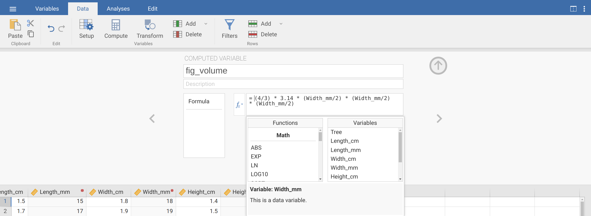
Figure 8.7: The jamovi toolbar where the tab ‘Data’ is selected. The box below shows the new computed variable ‘fig_volume’, which has been created by calculating the product of 4/3, 3.14, and Width_mm/2 three times.
Note that we can get the cube of ‘Width_mm’ more concisely by using the caret character (^).
That is, we would get the same answer shown in Figure 8.7 if we instead typed the below in the function box.
= (4/3) * 3.14 * (Width_mm/2)^3Note that the order of operations is important here, which is why there are parentheses around Width_mm/2. This calculation needs to be done before taking the value to the power of 3.
If we instead had written, Width_mm/2^3, then jamovi would first take the cube of 2 \((2 \times 2 \times 2 = 8)\), then divided Width_mm by this value giving a different and incorrect answer.
When in doubt, it is always useful to use parentheses to specify what calculations should be done first.
You now have the new column of data ‘fig_volume’. Remember that the calculations apply to the units too. The width of the fig was calculated in millimetres, but we have taken width to the power of 3 when calculating the volume. In the spaces below, find the mean, minimum, and maximum volumes of all figs and report them in the correct units.
Mean: ____________________________
Minimum: ____________________________
Maximum: ____________________________
Finally, it would be good to plot these newly calculated fig volume data. These data are continuous, so we can use a histogram to visualise the fig volume distribution. To make a histogram, go to the Exploration \(\to\) Descriptives window in jamovi (the same place where you found the mean, minimum, and maximum). Now, look on the lower left-hand side of the window and find the pull-down menu for ‘Plots’. Click ‘Plots’, and you should see several different plotting options. Check the option for ‘Histogram’ and see the new histogram plotted in the window to the right. Draw a rough sketch of the histogram in the area below.
We should save the file that we have been working on. There are two ways to save a file in jamovi, and it is a good idea to save both ways. The first way is to use jamovi’s own (binary) file type, which has the extension OMV. This will not only save the data (including the calculated variables created within jamovi), but also any analyses that we have done (e.g., calculation of minimums, maximums, and means) or graphs that we have made (e.g., the histogram). To do this, click on the three horizontal lines in the upper left of the jamovi toolbar, then select ‘Save As’. Choose an appropriate name (e.g., ‘chapter_8_exercises.omv’), then save the file in a location where you know that you will be able to find it again. Like all binary files, an OMV file cannot be opened as plain text. Hence, it might be a good idea to save the dataset as a CSV file (note, this will not save any of the analyses or graphs). To do this, click on the three horizontal lines in the upper left of the toolbar again, but this time click ‘Export’. Give the file an appropriate name (e.g., ‘chapter_8_dataset’), then choose ‘CSV’ from the pull-down menu below. Make sure to choose a save location that you know you will be able to find again (to navigate through file directories, click ‘Browse’ in the upper right). To save, click on ‘Export’ in the upper right.
8.4 Summary
You should now know some of the basic tools for working with data, calculating some simple descriptive statistics, plotting a histogram, and saving output and data in jamovi. These skills will be used throughout the book, so it is important to be comfortable with them as the analyses become more complex.