Chapter 18 Confidence intervals
In Chapter 16, we saw how it is possible to calculate the probability of sampling values from a specific interval of the normal distribution (e.g., the probability of sampling a value within 1 standard deviation of the mean). In this chapter, we will see how to apply this knowledge to calculating intervals that express confidence in the mean value of a population.
Remember that we almost never really know the true mean value of a population, \(\mu\). Our best estimate of \(\mu\) is the mean that we have calculated from a sample, \(\bar{x}\) (see Chapter 4 for a review of the difference between populations and samples). But how good of an estimate is \(\bar{x}\) of \(\mu\), really? Since we cannot know \(\mu\), one way of answering this question is to find an interval that expresses a degree of confidence about the value of \(\mu\). The idea is to calculate two numbers that we can say with some degree of confidence that \(\mu\) is between (i.e., a lower confidence interval and an upper confidence interval). The wider this interval is, the more confident that we can be that the true mean \(\mu\) is somewhere within it. The narrower the interval is, the less confident we can be that our confidence intervals (CIs) contain \(\mu\).
Confidence intervals are notoriously easy to misunderstand. I will explain this verbally first, focusing on the general ideas rather than the technical details. Then I will present the calculations before coming back to their interpretation again. The idea follows a similar logic to the standard error from Chapter 12.
Suppose that we want to know the mean body mass of all domestic cats (Figure 18.1). We cannot weigh every living cat in the world, but maybe we can find enough to get a sample of 20. From these 20 cats, we want to find some interval of masses (e.g., 3.9–4.3 kg) within which the true mean mass of the population is contained. The only way to be 100% certain that our proposed interval definitely contains the true mean would be to make the interval absurdly large. Instead, we might more sensibly ask what the interval would need to be to contain the mean with 95% confidence. What does ‘with 95% confidence’ actually mean? It means that when we do the calculation to get the interval, the true mean should be somewhere within the interval 95% of the time that a sample is collected.

Figure 18.1: Two domestic cats sitting side by side with much different body masses.
In other words, if we were to go back out and collect another sample of 20 cats, and then another, and another (and so forth), calculating 95% CIs each time, then in 95% of our samples the true mean will be within our CIs (meaning that 5% of the time it will be outside the CIs). Note that this is slightly different than saying that there is a 95% probability that the true mean is between our CIs.25 Instead, the idea is that if we were to repeatedly resample from a population and calculate CIs each time, then 95% of the time the true mean would be within our CIs (Sokal & Rohlf, 1995). If this idea does not make sense at first, that is okay. The calculation is actually relatively straightforward, and we will come back to the statistical concept again afterwards to interpret it. First, we will look at CIs assuming a normal distribution, then the separate case of a binomial distribution.
18.1 Normal distribution CIs
Remember from the Central Limit Theorem in Chapter 16 that as our sample size \(N\) increases, the distribution of our sample mean \(\bar{x}\) will start looking more and more like a normal distribution. Also from Chapter 16, we know that we can calculate the probability associated with any interval of values in a normal distribution. For example, we saw that about 68.2% of the probability density of a normal distribution is contained within one standard deviation of the mean. We can use this knowledge from Chapter 16 to set confidence intervals for any percentage of values around the sample mean (\(\bar{x}\)) using a standard error (SE) and z-score (\(z\)). Confidence intervals include two numbers. The lower confidence interval (LCI) is below the mean, and the upper confidence interval (UCI) is above the mean. Here is how they are calculated,
\[LCI = \bar{x} - (z \times SE),\]
\[UCI = \bar{x} + (z \times SE).\]
Note that the equations are the same, except that for the LCI, we are subtracting \(z \times SE\), and for the UCI we are adding it. The specific value of \(z\) determines the confidence interval that we are calculating. For example, about 95% of the probability density of a standard normal distribution lies between \(z = -1.96\) and \(z = 1.96\) (Figure 18.2). Hence, if we use \(z = 1.96\) to calculate LCI and UCI, we would be getting 95% confidence intervals around our mean (an interactive application26 helps visualise the relationship between probability intervals and z-scores more generally).
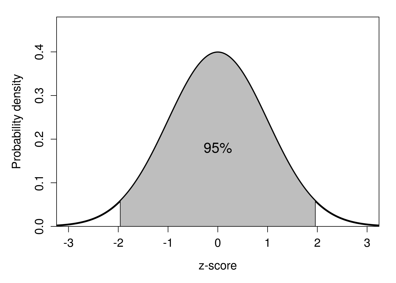
Figure 18.2: Standard normal probability distribution showing 95% of probability density surrounding the mean.
Now suppose that we want to calculate 95% CIs around the sample mean of our \(N = 20\) domestic cats from earlier. We find that the mean body mass of cats in our sample is \(\bar{x} = 4.1\) kg, and that the standard deviation is \(s = 0.6\) kg (suppose that we are willing to assume, for now, that \(s = \sigma\), that is, we know the true standard deviation of the population). Remember from Chapter 12 that the sample standard error can be calculated as \(s / \sqrt{N}\). Our lower 95% confidence interval is therefore,
\[LCI_{95\%} = 4.1 - \left(1.96 \times \frac{0.6}{\sqrt{20}}\right) = 3.837\]
Our upper 95% confidence interval is,
\[UCI_{95\%} = 4.1 + \left(1.96 \times \frac{0.6}{\sqrt{20}}\right) = 4.363\]
Our 95% CIs are therefore \(LCI = 3.837\) and \(UCI = 4.363\). We can now come back to the statistical concept of what this actually means. If we were to go out and repeatedly collect new samples of 20 cats, and do the above calculations each time, then 95% of the time our true mean cat body mass would be somewhere between the LCI and UCI.
The 95% confidence intervals are the most commonly used in the biological and environmental sciences. In other words, we accept that about 5% of the time (1 in 20 times), our confidence intervals will not contain the true mean that we are trying to estimate. Suppose, however, that we wanted to be a bit more cautious. We could calculate 99% CIs, that is, CIs that contain the true mean in 99% of samples. To do this, we just need to find the z-score that corresponds with 99% of the probability density of the standard normal distribution. This value is about \(z = 2.58\), which we could find with an interactive application, a z table, some maths, or a quick online search27. Consequently, the lower 99% confidence interval for our example of cat body masses would be,
\[LCI_{99\%} = 4.1 - \left(2.58 \times \frac{0.6}{\sqrt{20}}\right) = 3.754\]
Our upper 99% confidence interval is,
\[UCI_{99\%} = 4.1 + \left(2.58 \times \frac{0.6}{\sqrt{20}}\right) = 4.446\]
Notice that the confidence intervals became wider around the sample mean. The 99% CI is now 3.754–4.446, while the 95% CI was 3.837–4.363. This is because if we want to be more confident about our interval containing the true mean, we need to make a bigger interval.
We could make CIs using any percentage that we want, but in practice it is very rare to see anything other than 90% (\(z = 1.65\)), 95% (\(z = 1.96\)), or 99% (\(z = 2.58\)). It is useful to see what these different intervals look like when calculated from actual data (an interactive application28 illustrates CIs on a histogram). Unfortunately, the CI calculations from this section are a bit of an idealised situation. We assumed that the sample means are normally distributed around the population mean. While we know that this should be the case as our sample size increases, it is not quite true when our sample is small. In practice, what this means is that our z-scores are usually not going to be the best values to use when calculating CIs, although they are often good enough when a sample size is large29. We will see what to do about this in Chapter 19, but first we turn to the special case of how to calculate CIs from binomial proportions.
18.2 Binomial distribution CIs
For a binomial distribution, our data are counts of successes and failures (see Chapter 15). For example, we might flip a coin 40 times and observe 22 heads and 18 tails. Suppose that we do not know in advance the coin is fair, so we cannot be sure that the probability of it landing on heads is \(p = 0.5\). From our collected data, our estimated probability of landing on heads is, \(\hat{p} = 22/40 = 0.55\).30 But how would we calculate the CIs around this estimate? There are multiple ways to calculate CIs around proportions. One common method relies on a normal approximation, that is, approximating the discrete counts of the binomial distribution using the continuous normal distribution. For example, we can note that the variance of \(p\) for a binomial distribution is \(\sigma^{2} = p\left(1 - p\right)\) (Box et al., 1978; Sokal & Rohlf, 1995).31 This means that the standard deviation of \(p\) is \(\sigma = \sqrt{p\left(1 - p\right)}\), and \(p\) has a standard error,
\[\mathrm{SE}(p) = \sqrt{\frac{p\left(1 - p\right)}{N}}.\]
We could then use this standard error in the same equation from earlier for calculating CIs. For example, if we wanted to calculate the lower 95% CI for \(\hat{p} = 0.55\),
\[LCI_{95\%} = 0.55 - 1.96 \sqrt{\frac{0.55\left(1 - 0.55\right)}{40}} = 0.396\]
Similarly, to calculate the upper 95% CI,
\[UCI_{95\%} = 0.55 + 1.96 \sqrt{\frac{0.55\left(1 - 0.55\right)}{40}} = 0.704.\]
Our conclusion is that, based on our sample, 95% of the time we flip a coin 40 times, the true mean \(p\) will be somewhere between 0.396 and 0.704. These are quite wide CIs, which suggests that our flip of \(\hat{p} = 0.55\) would not be particularly remarkable even if the coin was fair (\(p = 0.5\)).32 This CI is called the Wald interval. It is easy to calculate, and is instructive for showing another way that CIs can be calculated. But it does not actually do a very good job of accurately producing 95% CIs around a proportion, especially when our proportion is very low or high (Andersson, 2023; Schilling & Doi, 2014).
In fact, there are many different methods proposed to calculate binomial CIs, and a lot of statistical research has been done to compare and contrast these methods (Reed, 2007; Schilling & Doi, 2014; Thulin, 2014). Jamovi uses Clopper-Pearson CIs (Clopper & Pearson E. S., 1934). Instead of relying on a normal approximation, the Clopper-Pearson method uses the binomial probability distribution (see Chapter 15) to build CIs. This is what is known as an ‘exact method’. Clopper-Pearson CIs tend to err on the side of caution (they are often made wider than necessary), but they are a much better option than Wald CIs (Reed, 2007).
References
The reason that these two ideas are different has to do with the way that probability is defined in the frequentist approach to statistics (see Chapter 15). With this approach, there is no way to get the probability of the true mean being within an interval, strictly speaking. Other approaches to probability, such as Bayesian probability, do allow you to build intervals in which the true mean is contained with some probability. These are called ‘credible intervals’ rather than ‘confidence intervals’ (e.g., Ellison, 2004). The downside to credible intervals (or not, depending on your philosophy of statistics) is that Bayesian probability is at least partly subjective, i.e., based in some way on the subjective opinion of the individual researcher.↩︎
While it is always important to be careful when searching, typing ‘z-score 99% confidence interval’ will almost always get the intended result.↩︎
What defines a ‘small’ or a ‘large’ sample is a bit arbitrary. A popular suggestion (e.g., Sokal & Rohlf, 1995, p. 145) is that any \(N < 30\) is too small to use z-scores, but any cut-off \(N\) is going to be somewhat arbitrary. Technically, the z-score is not completely accurate until \(N \to \infty\), but for all intents and purposes, it is usually only trivially inaccurate for sample sizes in the hundreds. Fortunately, you do not need to worry about any of this when calculating CIs from continuous data in jamovi because jamovi applies a correction for you, which we will look at in Chapter 19.↩︎
The hat over the p, (\(\hat{p}\)) is just being used here to indicate the estimate of \(P(heads)\), rather than the true \(P(heads)\).↩︎
Note, the variance of total successes is simply \(np\left(1 - p\right)\), i.e., just multiply the variance of \(p\) by \(n\).↩︎
You might ask, why are we doing all of this for the binomial distribution? The central limit theorem is supposed to work for the mean of any distribution, so should that not include the distribution of \(p\) too? Can we not just indicate success (heads) with a 1 and failures (tails) with a 0, then estimate the standard error of 22 values of 1 and 18 values of 0? Well, yes! That actually does work and gives an estimate of 0.079663, which is very close to the \(\sqrt{\hat{p}(1-\hat{p})/N} = 0.078661\). The problem arises when the sample size is low, or when \(p\) is close to 0 or 1, and we are trying to map the z-score to probability density.↩︎