Chapter 11 Measures of central tendency
Summary statistics describe properties of data in a single number (e.g., mean), or a set of numbers (e.g., quartiles). This chapter focuses on summary statistics that describe the centre of a distribution. It also introduces quantiles, which divide a distribution into different percentages of the data (e.g., lowest 50% or highest 75%). Throughout this section, verbal and mathematical explanations of summary statistics will be presented alongside histograms or boxplots that convey the same information. The point of doing this is to help connect the two ways of summarising the data. All of the summary statistics that follow describe calculations for a sample and are therefore estimates of the true values in a population. Recall from Chapter 4 the difference between a population and a sample. This book focuses on statistical techniques, not statistical theory, so summary statistics will just focus on how to estimate statistics from sampled data instead of how statistics are defined mathematically7.
11.1 The mean
The arithmetic mean (hereafter just the mean8) of a sample is one of the most commonly reported statistics when communicating information about a dataset. The mean is a measure of central tendency, so it is located somewhere in the middle of a distribution. Figure 11.1 shows the same histogram of fig fruit widths shown in Figure 10.1, but with an arrow indicating where the mean of the distribution is located.
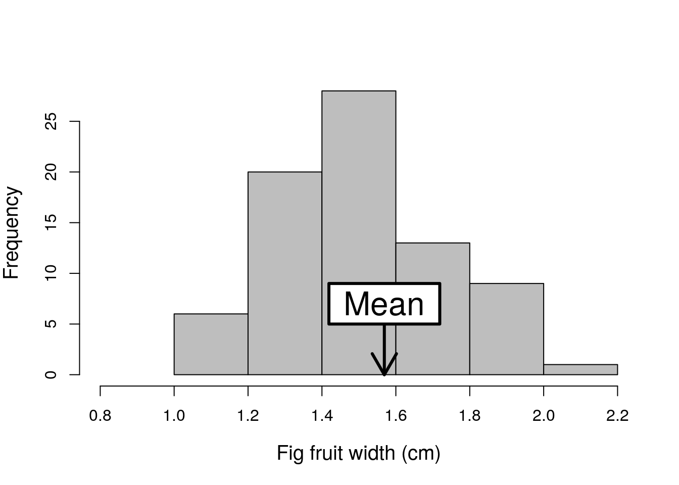
Figure 11.1: Example histogram fig fruit width (cm) using data from 78 fig fruits collected in 2010 from Baja, Mexico. The mean of the distribution is indicated with an arrow.
The mean is calculated by adding up the values of all of the data and dividing this sum by the total number of data (Sokal & Rohlf, 1995). This is a fairly straightforward calculation, so we can use the mean as an example to demonstrate some new mathematical notation that will be used throughout the book. We will start with a concrete example with actual numbers, then end with a more abstract equation describing how any sample mean is calculated. The notation might be a bit confusing at first, but learning it will make understanding statistical concepts easier later in the book. There are a lot of equations in what follows, but this is because I want to explain what is happening as clearly as possible, step by step. We start with the following eight values.
4.2, 5.0, 3.1, 4.2, 3.8, 4.6, 4.0, 3.5To calculate the mean of a sample, we just need to add up all of the values and divide by 8 (the total number of values),
\[\bar{x} = \frac{4.2 + 5.0 + 3.1 + 4.2 + 3.8 + 4.6 + 4.0 + 3.5}{8}.\]
Note that I have used the symbol \(\bar{x}\) to represent the mean of \(x\), which is a common notation (Sokal & Rohlf, 1995). In the example above, \(\bar{x} = 4.05\).
Writing the full calculation above is not a problem because we only have 8 points of data. But sample sizes are often much larger than 8. If we had a sample size of 80 or 800, then there is no way that we could write down every number to show how the mean is calculated. One way to get around this is to use ellipses and just show the first and last couple of numbers,
\[\bar{x} = \frac{4.2 + 5.0 + ... + 4.0 + 3.5}{8}.\]
This is a more compact, and perfectly acceptable, way to write the sample mean. But it is often necessary to have an even more compact way of indicating the sum over a set of values (i.e., top of the fraction above). To do this, each value can be symbolised by an \(x\), with a unique subscript \(i\), so that \(x_{i}\) corresponds to a specific value in the list above. The usefulness of this notation, \(x_{i}\), will become clear soon. It takes some getting used to, but Table 11.1 shows each symbol with its corresponding value to make it more intuitive.
| Symbol | \(x_{1}\) | \(x_{2}\) | \(x_{3}\) | \(x_{4}\) | \(x_{5}\) | \(x_{6}\) | \(x_{7}\) | \(x_{8}\) |
|---|---|---|---|---|---|---|---|---|
| Value | 4.2 | 5.0 | 3.1 | 4.2 | 3.8 | 4.6 | 4.0 | 3.5 |
Note that we can first replace the actual values with their corresponding \(x_{i}\), so the mean can be written as,
\[\bar{x} = \frac{x_{1} + x_{2} + x_{3} + x_{4} + x_{5} + x_{6} + x_{7} + x_{8}}{8}.\] Next, we can rewrite the top of the equation in a different form using a summation sign,
\[\sum_{i = 1}^{8}x_{i} = x_{1} + x_{2} + x_{3} + x_{4} + x_{5} + x_{6} + x_{7} + x_{8}.\] Like the use of \(x_{i}\), the summation sign \(\sum\) takes some getting used to, but here it just means ‘sum up all of the \(x_{i}\) values’. You can think of it as a big ‘S’ that just says ‘sum up’. The bottom of the S tells you the starting point, and the top of it tells you the ending point, for adding numbers. Verbally, we can read this as saying, ‘starting with \(i = 1\), add up all of the \(x_{i}\) values until \(i = 8\)’. We can then replace the long list of \(x\) values with a summation,
\[\bar{x} = \frac{\sum_{i = 1}^{8}x_{i}}{8}.\]
This still looks a bit messy, so we can rewrite the above equation. Instead of dividing the summation by 8, we can multiply it by 1/8, which gives us the same answer,
\[\bar{x} = \frac{1}{8}\sum_{i = 1}^{8}x_{i}.\]
There is one more step. We have started with 8 actual values and ended with a compact and abstract equation for calculating the mean. But if we want a general description for calculating any mean, then we need to account for sample sizes not equal to 8. To do this, we can use \(N\) to represent the sample size. In our example, \(N = 8\), but it is possible to have a sample size be any finite value above zero. We can therefore replace 8 with \(N\) in the equation for the sample mean,
\[\bar{x} = \frac{1}{N}\sum_{i = 1}^{N}x_{i}.\]
There we have it. Verbally, the above equation tells us to multiply \(1/N\) by the sum of all \(x_{i}\) values from 1 to \(N\). This describes the mean for any sample that we might collect.
11.2 The mode
The mode of a dataset is simply the value that appears most often. As a simple example, we can again consider the sample dataset of 8 values.
4.2, 5.0, 3.1, 4.2, 3.8, 4.6, 4.0, 3.5In this dataset, the values 5.0, 3.1, 3.8, 4.6, 4.0, and 3.5 are all represented once. But the value 4.2 appears twice, once in the first position and once in the fourth position. Because 4.2 appears most frequently in the dataset, it is the mode of the dataset.
Note that it is possible for a dataset to have more than one mode. Also, somewhat confusingly, distributions that have more than one peak are often described as multimodal, even if the peaks are not of the same height (Sokal & Rohlf, 1995). For example, the histogram in Figure 11.2 might be described as bimodal because it has two distinct peaks (one around 10 and the other around 14), even though these peaks are not the same size.
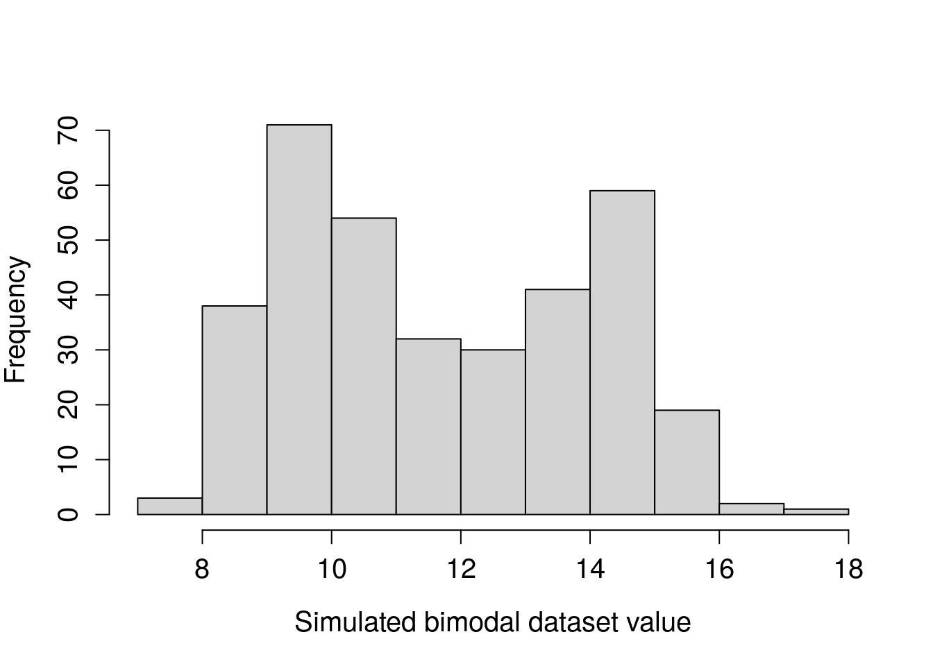
Figure 11.2: Example histogram of a hypothetical dataset that has a bimodal distribution.
In very rare cases, data might have a U-shape. The lowest point of the U would then be described as the antimode (Sokal & Rohlf, 1995).
11.3 The median and quantiles
The median of a dataset is the middle value when the data are sorted. More technically, the median is defined as the value that has the same number of lower and higher values than it (Sokal & Rohlf, 1995). If there is an odd number of values in the dataset, then finding the median is often easy. For example, the median of the values {8, 5, 3, 2, 6} is 5. This is because if we sort the values from lowest to highest (2, 3, 5, 6, 8), the value 5 is exactly in the middle. It gets more complicated for an even number of values, such as the sample dataset used for explaining the mean and mode.
4.2, 5.0, 3.1, 4.2, 3.8, 4.6, 4.0, 3.5We can order these values from lowest to highest.
3.1, 3.5, 3.8, 4.0, 4.2, 4.2, 4.6, 5.0Again, there is no middle value here. But we can find a value that has the same number of lower and higher values. To do this, we just need to find the mean of the middle 2 numbers, in this case 4.0 and 4.2, which are in positions 4 and 5, respectively. The mean of 4.0 and 4.2 is \((4.0 + 4.2)/2 = 4.1\), so 4.1 is the median value.
The median is a type of quantile. A quantile divides a sorted dataset into different percentages that are lower or higher than it. Hence, the median could also be called the 50% quantile because 50% of values are lower than the median and 50% of values are higher than it. Two other quantiles besides the median are also noteworthy. The first quartile (also called the ‘lower quartile’) defines the value for which 25% of values are lower and 75% of values are higher. The third quartile (also called the ‘upper quartile’) defines the value for which 75% of values are lower and 25% of values are higher. Sometimes this is easy to calculate. For example, if there are only five values in a dataset, then the lower quartile is the number in the second position when the data are sorted because 1 value (25%) is below it and 3 values (75%) are above it. For example, for the values {1, 3, 4, 8, 9}, the value 3 is the first quartile and 8 is the third quartile.
In some cases, it is not always this clear. We can show how quantiles get more complicated using the same 8 values as above where the first quartile is somewhere between 3.5 and 3.8.
3.1, 3.5, 3.8, 4.0, 4.2, 4.2, 4.6, 5.0There are at least nine different ways to calculate the first quartile in this case, and different statistical software packages will sometimes use different default methods (Hyndman & Fan, 1996). One logical way is to calculate the mean between the second (3.5) and third (3.8) position as you would do for the median (Rowntree, 2018), \((3.5 + 3.8) / 2 = 3.65\). Jamovi uses a slightly more complex method, which will give a value of \(3.725\) (The jamovi project, 2024).
It is important to emphasise that no one way of calculating quantiles is the one and only correct way. Statisticians have just proposed different approaches to calculating quantiles from data, and these different approaches sometimes give slightly different results. This can be unsatisfying when first learning statistics because it would be nice to have a single approach that is demonstrably correct, i.e., the right answer under all circumstances. Unfortunately, this is not the case here, nor is it the case for a lot of statistical techniques. Often there are different approaches to answering the same statistical question and no simple right answer. For this book, we will always report calculations of quantiles from jamovi. But it is important to recognise that different statistical tools might give different answers (Hyndman & Fan, 1996).