Chapter 1 Background mathematics
There are at least two types of mathematical challenges that come with first learning statistics. The first challenge is simply knowing the background mathematics upon which many statistical tools rely. Fortunately, while the theory underlying statistical techniques does rely on some quite advanced mathematics (e.g., see Mclean et al., 1991; Miller & Miller, 2004; Rencher, 2000), the application of standard statistical tools usually does not. This book focuses on the application of statistical techniques, so all that is required is a background in some fundamental mathematical concepts such as mathematical operations (addition, subtraction, multiplication, division, and exponents), simple algebra, and probability. This chapter will review mathematical operations and the symbols used to communicate them.
The second mathematical challenge that students face when learning statistics for the first time is a bit more subtle. Students with no statistical background sometimes have an expectation that statistics will be similar to previously learnt mathematical topics such as algebra, geometry, or trigonometry. In some ways, this is the case, but in a lot of ways statistics is a much different way of thinking than any of these topics. A lot of mathematical subjects focus on questions that have very clear right or wrong answers (or, at least, this is how they are often taught). If, for example, we are given the lengths of two sides of a right triangle, then we might be asked to calculate the hypotenuse of the triangle using Pythagorean theorem (\(a^{2} + b^{2} = c^{2}\), where c is the hypotenuse). If we know the length of the two sides, then the length of the hypotenuse has a clear correct answer (at least, on a Euclidean plane). In statistics, answers are not always so clear-cut. Statistics, by its very nature, deals with uncertainty. While all of the standard rules of mathematics still apply, statistical questions such as, ‘Can I use this statistical test on my data?’, ‘Do I have a large enough sample size?’, or even ‘Is my hypothesis well-supported?’ often do not have unequivocal ‘correct’ answers. Being a good statistician often means making well-informed, but ultimately at least somewhat subjective, judgements about how to make inferences from data.
For now, we will move on to looking at numbers and operations, logarithms, and order of operations. These topics will be relevant throughout the book, so it is important to understand them and be able to apply them when doing calculations.
1.1 Numbers and operations
Calculating statistics and reading statistical output requires some knowledge of numbers and basic mathematical operations. This section is a summary of the basic mathematical tools that will be used in introductory statistics. Much of this section is inspired by Courant et al. (1996) and chapter 2 of Pastor (2008). This section will focus on only the numbers and mathematical operations relevant to this book. The objective here is to present some very well-known ideas in an interesting way, and to intermix them with bits of information that might be new and interesting. For doing statistics, what you really need to know here are the operations and the notation, that is, how operations such as addition, multiplication, and exponents are calculated and represented mathematically.
We can start with the natural numbers, which are the kinds of numbers that can be counted using fingers, toothpicks, pebbles, or any discrete sets of objects.
\[1, 2, 3, 4, 5, 6, 7, 8, ...\]
There are an infinite number of natural numbers (we can represent the set of all of them using the symbol \(\mathbb{N}\)). For any given natural number, we can always find a higher natural number using the operation of addition. For example, a number higher than 5 can be obtained by simply adding 1 to it,
\[5 + 1 = 6.\]
This is probably not that much of a revelation, but it highlights why the natural numbers are countably infinite (for any number you can think of, \(N\), there is always a higher number \(N + 1\)). It also leads to a reminder about two other important mathematical symbols for this book (in addition to \(+\), which indicates addition), greater than (\(>\)) and less than (\(<\)). We know that the number 6 is greater than 5, and we express this mathematically as the inequality, \(6 > 5\). Note that the large end of the inequality faces the higher number, while the pointy end (i.e., the smaller end) faces the lower number. Inequalities are used regularly in statistics, e.g., to indicate when a probability of something is less than a given value (e.g., \(P < 0.05\), which can be read ‘P is less than 0.05’). We might also use the symbols \(\geq\) or \(\leq\) to indicate when something is greater than or equal to (\(\geq\)) or less than or equal to (\(\leq\)) a particular value. For example, \(x \geq 10\) indicates that some number \(x\) has a value of 10 or higher.
Whenever we add one natural number to another natural number, the result is another natural number, a sum (e.g., \(5 + 1 = 6\)). If we want to go back from the sum to one of the values being summed (i.e., get from \(6\) to \(5\)), then we need to subtract,
\[6 - 1 = 5.\]
This operation is elementary mathematics, but a subtle point that is often missed is that the introduction of subtraction creates the need for a broader set of numbers than the natural numbers. We call this broader set of numbers the integers (we can represent these using the symbol \(\mathbb{Z}\)). If, for example, we want to subtract 5 from 1, we get a number that cannot be represented on our fingers,
\[1 - 5 = -4.\]
The value \(-4\) is an integer (but not a natural number). Integers include 0 and all negative whole numbers,
\[..., -4, -3, -2, -1, 0, 1, 2, 3, 4, ...\]
Whenever we add or subtract integers, the result is always another integer.
Now, suppose we wanted to add the same value up multiple times. For example,
\[2 + 2 + 2 + 2 + 2 + 2 = 12.\]
The number 2 is being added 6 times in the equation above to get a value of 12. But we can represent this sum more easily using the operation of multiplication,
\[2 \times 6 = 12.\]
The 6 in the equation just represents the number of times that 2 is being added up.
The equation can also be written as \(2(6) = 12\), or sometimes, 2*6 = 12 (i.e., the asterisk is sometimes used to indicate multiplication).
Parentheses (i.e., round brackets) indicate multiplication when no other symbol separates them from a number.
This rule also applies to numbers that come immediately before variables.
For example, \(2x\) can be interpreted as two times x.
When multiplying integers, we always get another integer.
Multiplying two positive numbers always equals another positive number (e.g., \(2 \times 6 = 12\)).
Multiplying a positive and a negative number equals a negative number (e.g., \(-2 \times 6 = -12\)).
And multiplying two negative numbers equals a positive number (e.g., \(-2 \times -6 = 12\)).
There are multiple ways of thinking about why this last one is true (see, e.g., Askey, 1999 for one explanation), but for now we can take it as a given.
As with addition and subtraction, we need an operation that can go back from multiplied values (the product) to the numbers being multiplied. In other words, if we multiply to get \(2 \times 6 = 12\) (where 12 is the product), then we need something that goes back from 12 to 2. Division allows us to do this, such that \(12 \div 6 = 2\). In statistics, the symbol \(\div\) is rarely used, and we would more often express the calculation as either \(12/6 = 2\) or,
\[\frac{12}{6} = 2.\]
As with subtraction, there is a subtle point that the introduction of division requires a new set of numbers. If instead of dividing 6 into 12, we divided 12 into 6,
\[\frac{6}{12} = \frac{1}{2} = 0.5.\]
We now have a number that is not an integer. We therefore need a new broader set of numbers, the rational numbers (we can represent these using the symbol \(\mathbb{Q}\)). The rationals include all numbers that can be expressed as a ratio of integers. That is, \(p / q\), where both \(p\) and \(q\) are in the set \(\mathbb{Z}\).
We have one more set of operations relevant for introductory statistics. Recall that we introduced \(2 \times 6\) as a way to represent \(2 + 2 + 2 + 2 + 2 + 2\). We can apply the same logic to multiplying a number multiple times. For example, we might want to multiply the number 2 by itself 4 times,
\[2 \times 2 \times 2 \times 2 = 16.\]
We can represent this more compactly using an exponent, which is written as a superscript,
\[2^{4} = 16.\]
The 4 in the equation above indicates that the 2 should be multiplied 4 times to get 16. Sometimes this is also represented by a caret in writing or code, such that 2^4 = 16. Very occasionally, some authors will use two asterisks in a row, 2**4 = 16, probably because this is how exponents are represented in some statistical software and programming languages. One quick note that can be confusing at first is that a negative in the exponent indicates a reciprocal. For example,
\[2^{-4} = \frac{1}{16}.\]
This can sometimes be useful for representing the reciprocal of a number or unit in a more compact way than using a fraction (we will come back to this in Chapter 6).
As with addition and subtraction, and multiplication and division, we also need an operation to get back from the exponentiated value to the original number. That is, for \(2^{4} = 16\), there should be an operation that gets us back from 16 to 2. We can do this using the root of an equation,
\[\sqrt[4]{16} = 2.\]
The number under the radical symbol \(\sqrt{}\) (in this case 16) is the one that we are taking the root of, and the index (in this case 4) is the root that we are calculating. When the index is absent, we assume that it is 2 (i.e., a square root),
\[\sqrt[2]{16} = \sqrt{16} = 4.\]
Note that \(4^{2} = 16\) (i.e., 4 squared equals 16).
Instead of using the radical symbol, we could also use a fraction in the exponent. That is, instead of writing \(\sqrt[4]{16} = 2\), we could write \(16^{1/4} = 2\) or \(16^{1/2} = 4\). In statistics, however, the \(\sqrt{}\) is more often used. Either way, this yet again creates the need for an even broader set of numbers. This is because expressions such as \(\sqrt{2}\) do not equal any rational number. In other words, there are no integers \(p\) and \(q\) such that their ratio, \(p/q = \sqrt{2}\) (the proof for why is very elegant!). Consequently, we can say that \(\sqrt{2}\) is irrational (not in the colloquial sense of being illogical or unreasonable, but in the technical sense that it cannot be represented as a ratio of two integers). Irrational numbers cannot be represented as a ratio of integers, or with a finite or repeating decimal. Remarkably, the set of irrational numbers is larger than the set of rational numbers (i.e., rational numbers are countably infinite, while irrational numbers are uncountably infinite, and there are more irrationals; you do not need to know this or even believe it, but it is true!).
Perhaps the most famous irrational number is \(\pi\), which appears throughout science and mathematics and is most commonly introduced as the ratio of a circle’s circumference to its diameter. Its value is \(\pi \approx 3.14159\), where the symbol \(\approx\) means ‘approximately.’ Actually, the decimal expansion of \(\pi\) is infinite and non-repeating; the decimals go on forever and never repeat themselves in a predictable pattern. As of 2019, over 31 trillion (i.e., 31000000000000) decimals of \(\pi\) have been calculated (Yee, 2019).
The rational and irrational numbers together comprise a set of numbers called real numbers (we can represent these with the symbol \(\mathbb{R}\)), and this is where we will stop. This story of numbers and operations continues with imaginary and complex numbers (Courant et al., 1996; Pastor, 2008), but these are not necessary for introductory statistics.
1.2 Logarithms
There is one more important mathematical operation to mention that is relevant to introductory statistics. Logarithms are important functions, which will appear in multiple places (e.g., statistical transformations of variables). A logarithm tells us the exponent to which a number needs to be raised to get another number. For example,
\[10^{3} = 1000.\]
Verbally, 10 raised to the power of 3 equals 1000. In other words, we need to raise 10 to the power of 3 to get a value of 1000. We can express this using a logarithm,
\[\log_{10}\left(1000\right) = 3.\]
Again, the same relationship is expressed in \(10^{3} = 1000\) and \(\log_{10}(1000) = 3\). For the latter, we might say that the base 10 logarithm of 1000 is 3. This is actually extremely useful in mathematics and statistics. Mathematically, logarithms have the very useful property,
\[\log_{10}(ab) = \log_{10}(a) + \log_{10}(b).\]
Historically, this has been used to make calculations easier by converting multiplication to addition (Stewart, 2008). In statistics, and across the biological and environmental sciences, we often use logarithms when we want to represent something that changes exponentially on a more convenient scale. For example, suppose that we wanted to illustrate the change in global CO\(_{2}\) emissions over time (Friedlingstein et al., 2022). We could show year on the x-axis and emissions in billions of tonnes of CO\(_{2}\) on the y-axis (Figure 1.1).
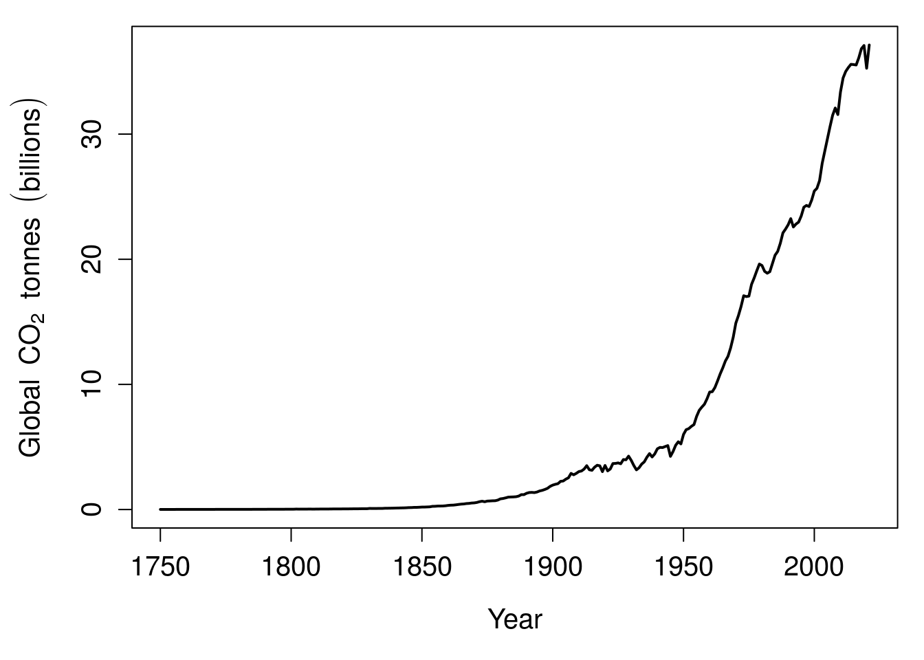
Figure 1.1: Global carbon dioxide emissions 1750–2021.
We can see from Figure 1.1 that global CO\(_{2}\) emissions go up exponentially over time, but this exponential relationship means that the y-axis has to cover a large range of values. This makes it difficult to see what is actually happening in the first 100 years. Are CO\(_{2}\) emissions increasing from 1750 to 1850, or do they stay about the same? If instead of plotting billions of tonnes of CO\(_{2}\) on the y-axis, we plotted the logarithm of these values, then the pattern in the first 100 years becomes a bit clearer (Figure 1.2).
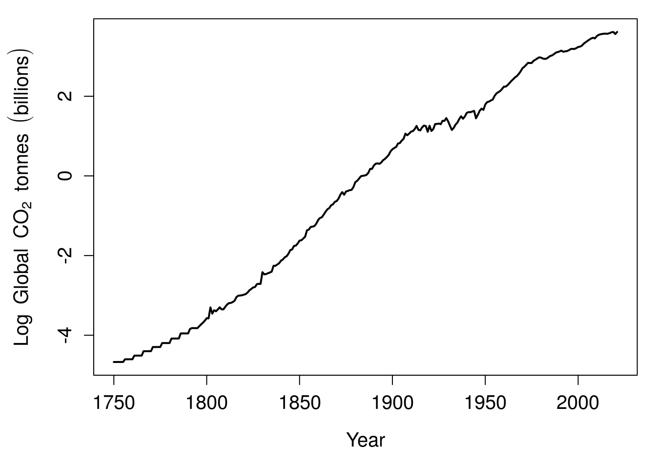
Figure 1.2: Natural logarithm of global carbon dioxide emissions 1750–2021.
It appears from the logged data in Figure 1.2 that global CO\(_{2}\) emissions were indeed increasing from 1750 to 1850. Note that Figure 1.2 presents the natural logarithm of CO\(_{2}\) emissions on the y-axis. The natural logarithm uses Euler’s number, \(e \approx 2.718282\), as a base. Euler’s number \(e\) is an irrational number (like \(\pi\)), which corresponds to the intrinsic rate of increase of a population’s size in ecology (Gotelli, 2001), or, in banking, interest compounded continuously (like \(\pi\), \(e\) actually shows up in a lot of different places throughout science and mathematics). We probably could have just as easily used 10 as a base, but \(e\) is usually the default base to use in science (bases 10 or 2 are also often used). Note that we can convert back to the non-logged scale by raising numbers to the power of \(e\). For example, \(e^{-4} \approx 0.018\), \(e^{-2} \approx 0.135\), \(e^{0} = 1\), and \(e^{2} = 7.390\).
1.3 Order of operations
Every once in a while, a maths problem like the one below seems to go viral online,
\[x = 8 \div 2\left(2+2\right).\]
Depending on the order in which calculations are made, some people will conclude that \(x = 16\), while others conclude that \(x = 1\) (Chernoff & Zazkis, 2022). The confusion is not caused by the above calculation being difficult, but by peoples’ differences in interpreting the rules for the order by which calculations should be carried out. If we first divide 8/2 to get 4, then multiply by (2 + 2), we get 16. If we first multiply 2 by (2 + 2) to get 8, then divide, we get 1. The truth is that even if there is a ‘right’ answer here (Chernoff & Zazkis, 2022), the equation could be written more clearly. We might, for example, rewrite the above to more clearly express the intended order of operations,
\[x = \frac{8}{2}\left(2 + 2\right) = 16.\]
We could write it a different way to express a different intended order of operations,
\[x = \frac{8}{2(2+2)} = 1.\]
The key point is that the order in which operations are calculated matters, so it is important to write equations clearly, and to know the order of operations to calculate an answer correctly. By convention, there are some rules for the order in which calculations should proceed.
- Anything within parentheses should always be calculated first.
- Exponents and radicals should be applied second.
- Multiplication and division should be applied third.
- Addition and subtraction should be done last.
These conventions are not really rooted in anything fundamental about numbers or operations (i.e., we made these rules up), but there is a logic to them. First, parentheses are a useful tool for being unequivocal about the order of operations. We could, for example, always be completely clear about the order to calculate by writing something like \((8/2) \times (2+2)\) or \(8 / (2(2 + 2))\), although this can get a bit messy. Second, rules 2–4 are ordered by the magnitude of operation effects; for example, exponents have a bigger effect than multiplication, which has a bigger effect than addition. In general, however, these are just standard conventions that need to be known for reading and writing mathematical expressions. In this book, you will not see something ambiguous like \(x = 8 \div 2\left(2+2\right)\), but you should be able to correctly calculate something like this,
\[x = 3^{2} + 2\left(1 + 3\right)^{2} - 6 \times 0.\]
First, remember that parentheses come first, so we can rewrite the above,
\[x = 3^{2} + 2\left(4\right)^{2} - 6 \times 0.\]
Exponents come next, so we can calculate those,
\[x = 9 + 2\left(16\right) - 6 \times 0.\]
Next comes multiplication and division,
\[x = 9 + 32 - 0.\]
Lastly, we calculate addition and subtraction,
\[x = 41.\]
In this book, you will very rarely need to calculate something with this many different steps. But you will often need to calculate equations like the one below,
\[x = 20 + 1.96 \times 2.1.\]
It is important to remember to multiply \(1.96 \times 2.1\) before adding 20. Getting the order of operations wrong will usually result in the calculation being completely off.
One last note is that when operations are above or below a fraction, or below a radical, then parentheses are implied. For example, we might have something like the fraction below,
\[x = \frac{2^{2} + 1}{3^{2} +2}.\]
Although rules 2–4 still apply, it is implied that there are parentheses around both the top (numerator) and bottom (denominator), so you can always read the above equation like this,
\[x = \frac{\left(2^{2} + 1\right)}{\left(3^{2} + 2\right)} = \frac{\left(4 + 1\right)}{\left(9 + 2\right)} = \frac{5}{11}.\]
Similarly, anything under the \(\sqrt{}\) can be interpreted as being within parentheses. For example,
\[x = \sqrt{3 + 4^{2}} = \sqrt{\left(3 + 4^{2} \right)} \approx 4.47.\]
This can take some getting used to, but with practice, it will become second nature to read equations with the correct order of operations.