Chapter 19 The t-interval
Chapter 15 introduced the binomial, Poisson, uniform, and normal distributions. In this chapter, I introduce another distribution, the t-distribution. Unlike the distributions of Chapter 15, the t-distribution arises from the need to make accurate statistical inferences, not from any particular kind of data (e.g., successes or failures in a binomial distribution, or events happening over time in a Poisson distribution). In Chapter 18, we calculated confidence intervals (CIs) using the normal distribution and z-scores. In doing so, we made the assumption that the sample standard deviation (\(s\)) was the same as the population standard deviation (\(\sigma\)), \(s = \sigma\). In other words, we assumed that we knew what \(\sigma\) was, which is almost never true. For large enough sample sizes (i.e., high \(N\)), this is not generally a problem, but for lower sample sizes we need to be careful.
If there is a difference between \(s\) and \(\sigma\), then our CIs will also be wrong. More specifically, the uncertainty between our sample estimate (\(s\)) and the true standard deviation (\(\sigma\)) is expected to increase the deviation of our sample mean (\(\bar{x}\)) from the true mean (\(\mu\)). This means that when we are using the sample standard deviation instead of the population standard deviation (which is pretty much always), the shape of the standard normal distribution from Chapter 18 (Figure 18.2) will be wrong. The correct shape will be ‘wider and flatter’ (Sokal & Rohlf, 1995), with more probability density at the extremes and less in the middle of the distribution (Box et al., 1978). What this means is that if we use z-scores when calculating CIs using \(s\), our CIs will not be wide enough, and we will think that we have more confidence in the mean than we really do. Instead of using the standard normal distribution, we need to use a t-distribution33.
The difference between the standard normal distribution and t-distribution depends on our sample size, \(N\). As \(N\) increases, we become more confident that the sample variance will be close to the true population variance (i.e., the deviation of \(s^{2}\) from \(\sigma^{2}\) decreases). At low \(N\), our t-distribution is much wider and flatter than the standard normal distribution. As \(N\) becomes large34, the t-distribution becomes basically indistinguishable from the standard normal distribution. For calculating CIs from a sample, especially for small sample sizes, it is therefore best to use t-scores instead of z-scores. The idea is the same; we are just multiplying the standard errors by a different constant to get our CIs. For example, in Chapter 18, we multiplied the standard error of 20 cat masses by \(z = 1.96\) because 95% of the probability density lies between \(z = -1.96\) and \(z = 1.96\) in the standard normal distribution. In truth, we should have multiplied by \(-2.093\) because we only had a sample size of \(N = 20\). Figure 19.1 shows the difference between the standard normal distribution and the more appropriate t-distribution35.
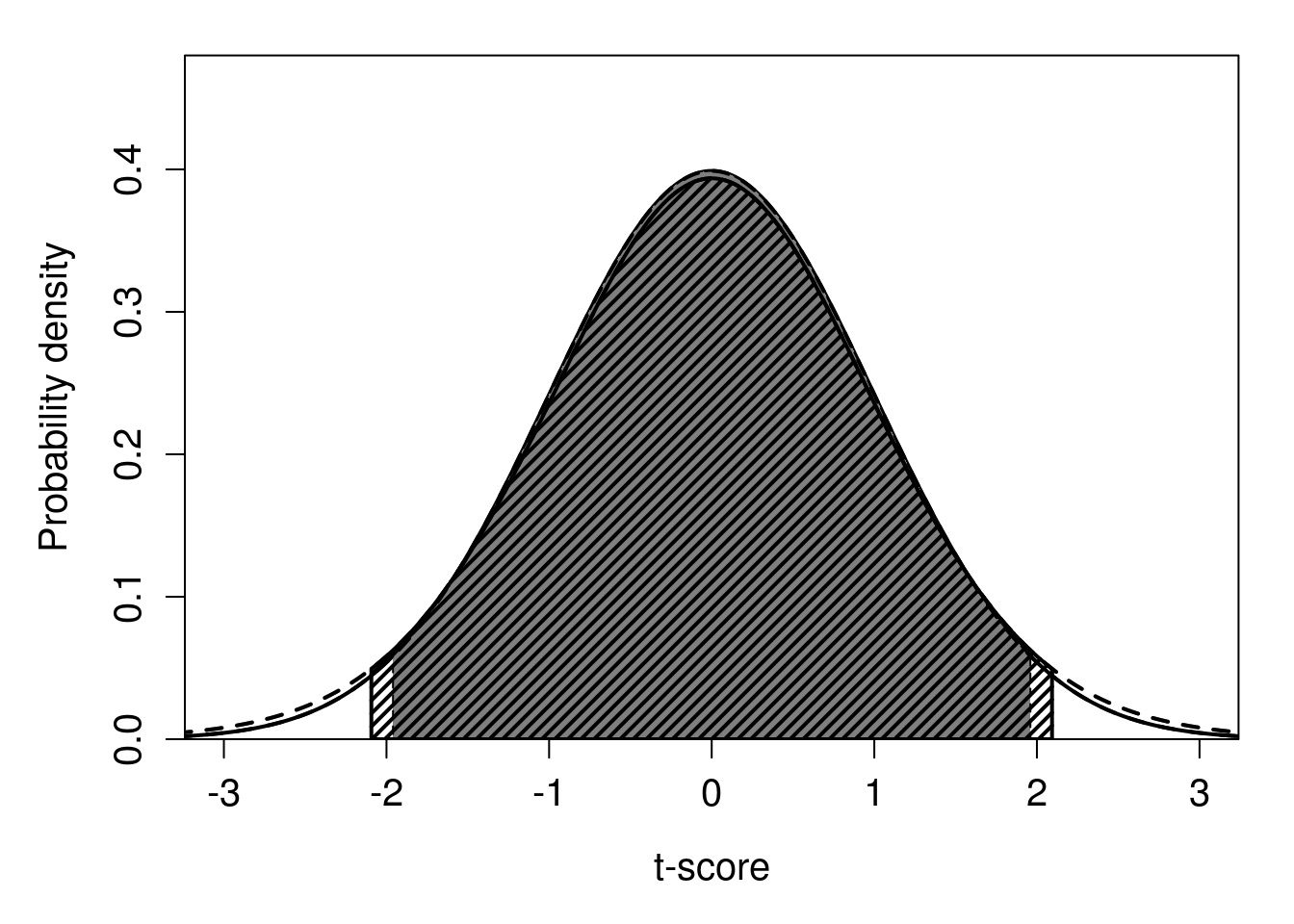
Figure 19.1: Standard normal probability distribution showing 95% of probability density surrounding the mean (dark grey shading). On top of the standard normal distribution in dark grey, hatched lines show a t-distribution with 19 degrees of freedom. Hatched lines indicate 95% of the probability density of the t-distribution.
Note that in Figure 19.1, a t-distribution with 19 degrees of freedom (\(df\)) is shown. The t-distribution is parameterised using df, and we lose a degree of freedom when calculating \(s^{2}\) from a sample size of \(N = 20\), so \(df = 20 - 1 = 19\) is the correct value (see Chapter 12 for explanation). For calculating CIs, df will always be \(N - 1\), and this will be taken care of automatically in jamovi36 (The jamovi project, 2024).
Recall from Chapter 18 that our body mass measurements of 20 cats had a sample mean of \(\bar{x} = 4.1\) kg and sample standard deviation of \(s = 0.6\) kg. We calculated the lower 95% CI to be \(LCI_{95\%} = 3.837\) and the upper 95% CI to be \(UCI_{95\%} = 4.363\). We can now repeat the calculation using the t-score 2.093 instead of the z-score 1.96. Our corrected lower 95% CI is,
\[LCI_{95\%} = 4.1 - \left(2.093 \times \frac{0.6}{\sqrt{20}}\right) = 3.819.\]
Our upper 95% confidence interval is,
\[UCI_{95\%} = 4.1 + \left(2.093 \times \frac{0.6}{\sqrt{20}}\right) = 4.381.\]
The confidence intervals have not changed too much. By using the t-distribution, the LCI changed from 3.837 to 3.819, and the UCI changed from 4.363 to 4.381. In other words, we only needed our CIs to be a bit wider (\(4.381 - 3.819 = 0.562\) for the using t-scores versus \(4.363 - 3.837 = 0.526\) using z-scores). This is because a sample size of 20 is already large enough for the t-distribution and standard normal distribution to be very similar (Figure 19.1). But for lower sample sizes and therefore fewer degrees of freedom, the difference between the shapes of these distributions gets more obvious (Figure 19.2).
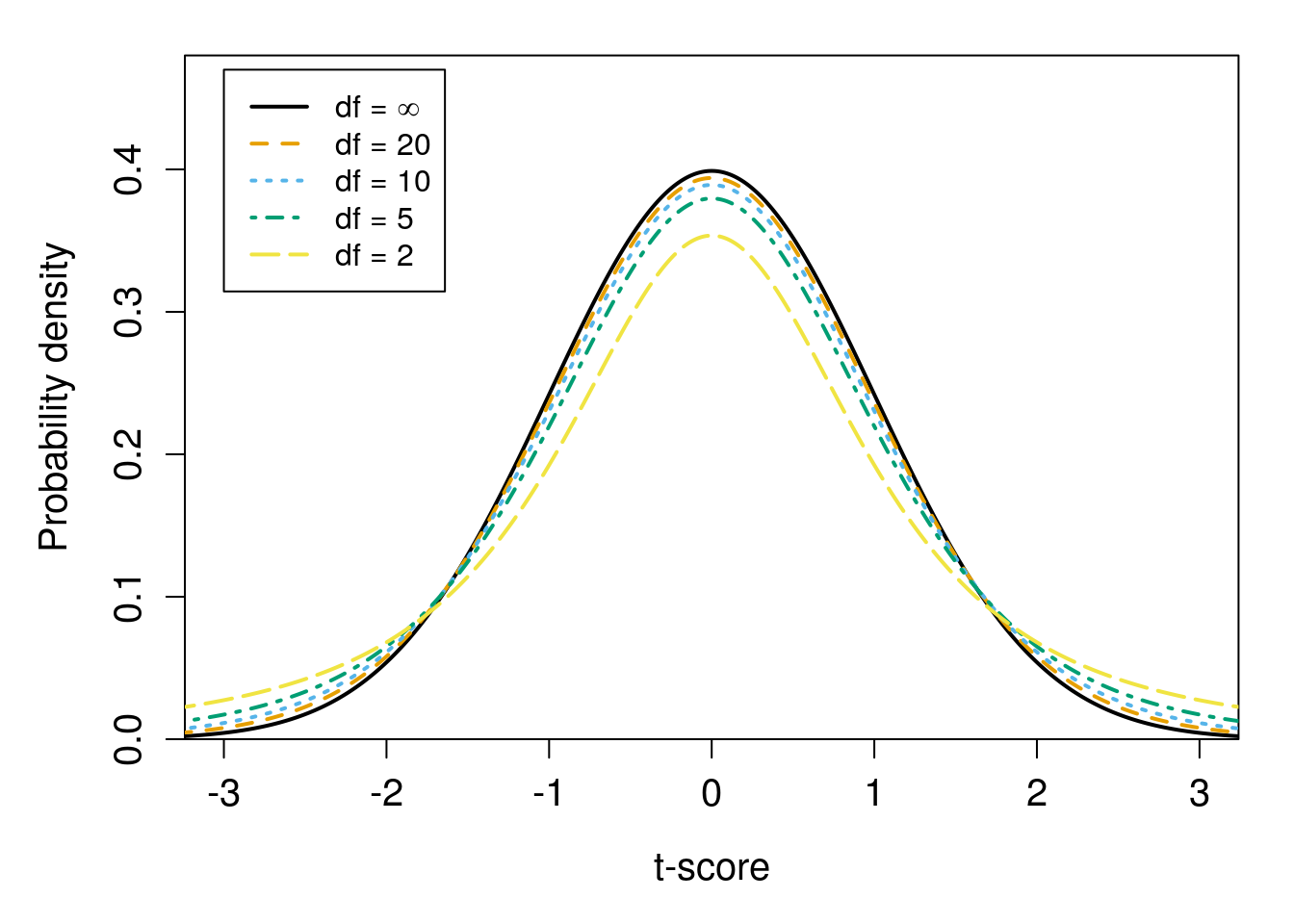
Figure 19.2: A t-distribution with infinite degrees of freedom (df) is shown in black; this distribution is identical to the standard normal distribution. Other t-distributions with the same mean and standard deviation, but different degrees of freedom, are indicated by curves of different line types.
The main point of Figure 19.2 is that as degrees of freedom decreases, the t-distribution becomes wider, with more probability density in the tails. Figure 19.2 is quite busy, so an interactive application37 can make visualising the t-distribution easier. The t-distribution is important throughout most of the rest of this book. It is not just used for calculating confidence intervals. The t-distribution also plays a critical role in hypothesis-testing, which is the subject of Chapter 22 and applied throughout the rest of the book. The t-distribution is therefore very important for understanding many statistical techniques.
References
This is also called the ‘Student’s t-distribution’. It was originally discovered by the head brewer of Guinness in Dublin in the early 20th century (Box et al., 1978). The brewer, W. S. Gosset, published under the pseudonym ‘A. Student’ because Guinness had a policy of not allowing employees to publish (Miller & Miller, 2004).↩︎
How large N needs to be for the t-distribution to considered close enough to the normal distribution is subjective. The two distributions get closer and closer as \(N \to \infty\), but Sokal & Rohlf (1995) suggest that they are indistinguishable for all intents and purposes once \(N > 30\). It is always safe to use the t-distribution when calculating confidence intervals, which is what all statistical programs such as jamovi will do by default, so there is no need to worry about these kinds of arbitrary cutoffs in this case.↩︎
We can define the t-distribution mathematically (Miller & Miller, 2004), but it is an absolute beast, \[f(t) = \frac{\Gamma\left(\frac{v + 1}{2} \right)}{\sqrt{\pi v} \Gamma{\left(\frac{v}{2}\right)}}\left(1 + \frac{t^{2}}{v} \right)^{-\frac{v + 1}{2}}.\] In this equation, \(v\) is the degrees of freedom. The \(\Gamma\left(\right)\) is called a ‘gamma function’, which is basically the equivalent of a factorial function, but for any number z (not just integers), such that \(\Gamma(z + 1) = \int_{0}^{\infty}x^{z}e^{-x}dx\) (where \(z > -1\), or, even more technically, the real part of \(z > -1\)). If z is an integer n, then \(\Gamma\left({n + 1}\right) = n!\) (Borowski & Borwein, 2005). What about the rest of the t probability density function? Why is it all so much? The reason is that it is the result of two different probability distributions affecting t independently, a standard normal distribution and a Chi-square distribution (Miller & Miller, 2004). We will look at the Chi-square in Chapter 29. Suffice to say that underlying mathematics of the t-distribution is not important for our purposes in applying statistical techniques.↩︎
Another interesting caveat, which jamovi will take care of automatically (so we do not actually have to worry about it), is that when we calculate \(s^{2}\) to map t-scores to probability densities in the t-distribution, we multiply the sum of squares by \(1/N\) instead of \(1/(N-1)\) (Sokal & Rohlf, 1995). In other words, we no longer need to correct the sample variance \(s^{2}\) to account for bias in estimating \(\sigma^{2}\) because the t-distribution takes care of this for us.↩︎