Chapter 24 Analysis of variance

An ANalysis Of VAriance (ANOVA) is, as the name implies, a method for analysing variances in a dataset. This is confusing, at first, because the most common application of an ANOVA is to test for differences among group means. That is, an ANOVA can be used to test the same null hypothesis as the independent samples Student’s t-test introduced in Section 22.2; are two groups sampled from a population that has the same mean? The t-test works fine when we have only two groups, but it does not work when there are three or more groups, and we want to know if the groups all have the same mean. An ANOVA can be used to test the null hypothesis that all groups in a dataset are sampled from a population with the same mean. For example, we might want to know if mean wing length is the same for five species of fig wasps sampled from the same area (Duthie et al., 2015). What follows is an explanation of why this can be done by looking at the variance within and between groups (note, ‘groups’ are also sometimes called ‘factors’ or ‘levels’). Groups are categorical data (see Chapter 5). In the case of the fig wasp example, the groups are the different species (Table 24.1).

TABLE 24.1 Wing lengths (mm) measured for five unnamed species of non-pollinating fig wasps collected from fig trees in 2010 near La Paz in Baja, Mexico.

Het1	Het2	LO1	SO1	SO2
2.122	1.810	1.869	1.557	1.635
1.938	1.821	1.957	1.493	1.700
1.765	1.653	1.589	1.470	1.407
1.700	1.547	1.430	1.541	1.378

Why is any of this necessary? If we want to know if the five species of fig wasps in Table 24.1 have the same mean wing length, can we not just use t-tests to compare the means between each species? There are a couple of problems with this approach. First, there are a lot of group combinations to compare (Het1 vs Het2, Het1 vs LO1, Het1 vs SO1, etc.). For the five fig wasp species in Table 24.1, there are 10 pair-wise combinations that would need to be tested. And the number of combinations grows exponentially⁵⁴ with each new group added to the dataset (Table 24.2).

TABLE 24.2 Number of individual t-tests that would need to be run to compare the means given different numbers of groups (e.g., if a dataset had measurements from 2–10 species).

Groups	2	3	4	5	6	7	8	9	10
Tests	1	3	6	10	15	21	28	36	45

Aside from the tedium of testing every possible combination of group means, there is a more serious problem having to do with the Type I error. Recall from Section 21.3 that a Type I error occurs when we rejected the null hypothesis (\(H_{0}\)) and erroneously conclude that \(H_{0}\) is false when it is actually true (i.e., a false positive). If we reject \(H_{0}\) at a threshold level of \(\alpha = 0.05\) (i.e., reject \(H_{0}\) when \(P < 0.05\), as usual), then we will erroneously reject the null hypothesis about 5% of the time that we run a statistical test and \(H_{0}\) is true. But if we run 10 separate t-tests to see if the fig wasp species in Table 24.1 have different mean wing lengths, then the probability of making an error increases considerably. The probability of erroneously rejecting at least 1 of the 10 null hypotheses increases from 0.05 to about 0.40. In other words, about 40% of the time, we would conclude that at least two species differ in their mean wing lengths⁵⁵ even when all species really do have the same wing length. This is not a mistake that we want to make, which is why we should first test if all of the means are equal:

• \(H_{0}:\) Mean species wing lengths are all the same
• \(H_{A}:\) Mean species wing lengths are not all the same

We can use an ANOVA to test the null hypothesis above against the alternative hypothesis. If we reject \(H_{0}\), then we can start comparing pairs of group means (more on this in Chapter 26).

How do we test the above \(H_{0}\) by looking at variances instead of means? Before getting into the details of how an ANOVA works, we will first look at the F-distribution. This is relevant because the test statistic calculated in an ANOVA is called an F-statistic, which is compared to an F-distribution in the same way that a t-statistic is compared to a t-distribution for a t-test (see Chapter 22).

24.1 F-distribution

If we want to test whether or not two variances are the same, then we need to know what the null distribution should be if two different samples came from a population with the same variance. The general idea is the same as it was for the distributions introduced in Section 15.4. For example, if we wanted to test whether or not a coin is fair, then we could flip it 10 times and compare the number of times it comes up heads to probabilities predicted by the binomial distribution when \(P(Heads) = 0.5\) and \(N = 10\) (see Section 15.4.1 and Figure 15.5). To test variances, we will calculate the ratio of variances (\(F\)), then compare it to the \(F\) probability density function⁵⁶. For example, the ratio of the variances for two samples, 1 and 2, is (Sokal & Rohlf, 1995),

\[F = \frac{\mathrm{Variance}\:1}{\mathrm{Variance}\:2}.\]

Note that if the variances of samples 1 and 2 are the exact same, then \(F = 1\). If the variances are very different, then \(F\) is either very low (if Variance 1 < Variance 2) or very high (if Variance 1 > Variance 2). To test the null hypothesis that samples 1 and 2 have the same variance, we therefore need to map the calculated \(F\) to the probability density of the F-distribution. Again, the general idea is the same as comparing a t-score to the t-distribution in Section 22.1. Recall that the shape of the t-distribution is slightly different for different degrees of freedom (\(df\)). As \(df\) increases, the t-distribution starts to resemble the normal distribution. For the F-distribution, there are actually two degrees of freedom to consider. One degree of freedom is needed for Variance 1, and a second degree of freedom is needed for Variance 2. Together, these two degrees of freedom will determine the shape of the F-distribution (Figure 24.1).

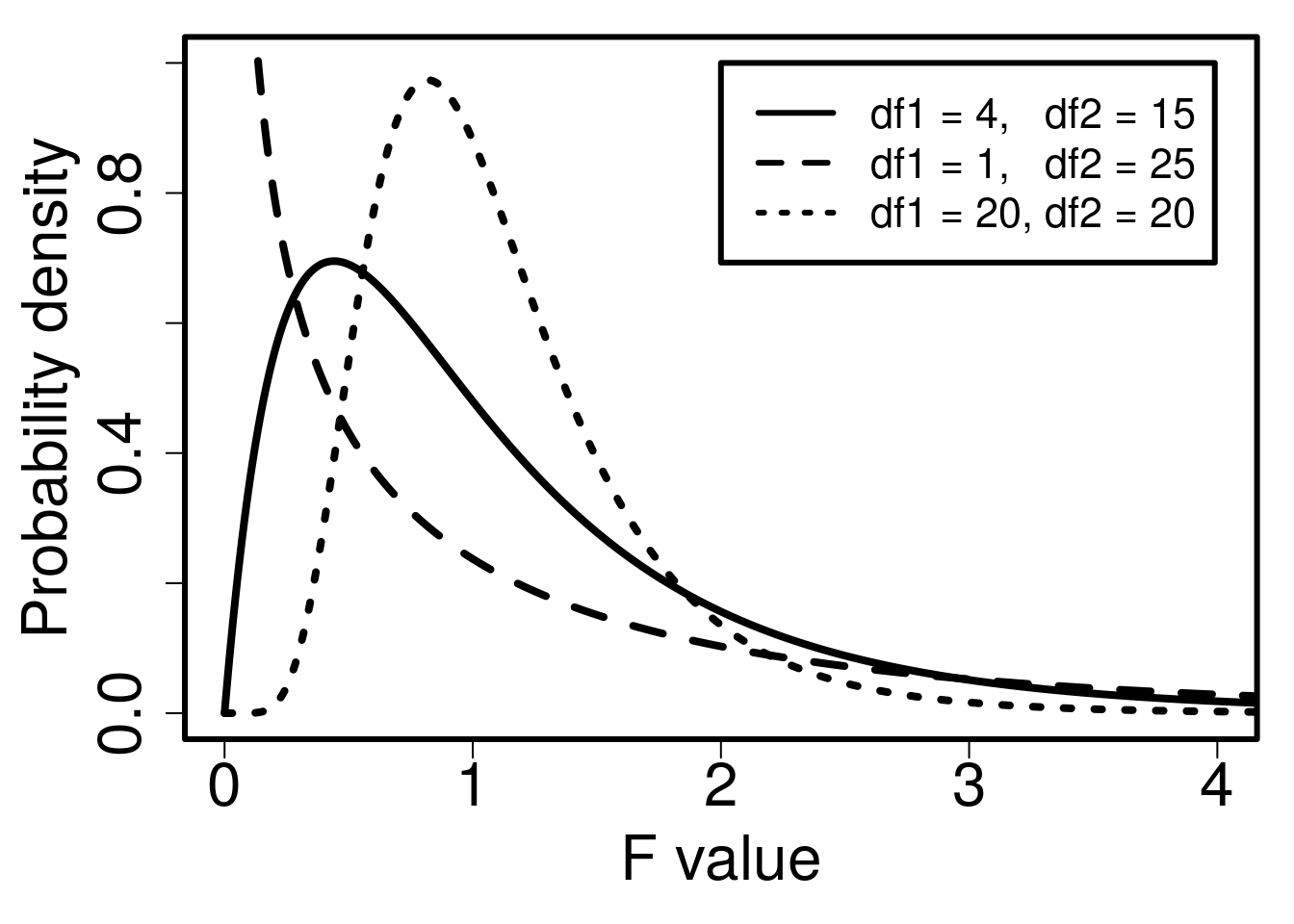
Figure 24.1: Probability density functions for three different F-distributions, each of which has different degrees of freedom for the variances in the numerator (df1) and denominator (df2).

Figure 24.1 shows an F-distribution for three different combinations of degrees of freedom. The F-distribution changes its shape considerably given different df values (visualising this is easier with an interactive application⁵⁷).

It is not necessary to memorise how the F-distribution changes with different degrees of freedom. The point is that the probability distribution changes given different degrees of freedom, and that the relationship between probability and the value on the x-axis (\(F\)) works like other distributions such as the normal or t-distribution. The entire area under the curve must sum to 1, and we can calculate the area above and below any \(F\) value (rather, we can get jamovi to do this for us). Consequently, we can use the F-distribution as the null distribution for the ratio of two variances. If the null hypothesis that the two variances are the same is true (i.e., \(F = 1\)), then the F-distribution gives us the probability of the ratio of two variances being as or more extreme (i.e., further from 1) than a specific value.

24.2 One-way ANOVA

We can use the F-distribution to test the null hypothesis mentioned at the beginning of the chapter (that fig wasp species have the same mean wing length). The general idea is to compare the mean variance among groups to the mean variance within groups, so our F value (i.e., ‘F-statistic’) is calculated,

\[F = \frac{\mathrm{Mean\:variance\:among\:\:groups}}{\mathrm{Mean\:variance\:within\:\:groups}}.\]

The rest of this section works through the details of how to calculate this F-statistic. It is easy to get lost in these details, but the calculations that follow do not need to be done by hand. As usual, jamovi will do all of this work for us (The jamovi project, 2024). The reason for going through the ANOVA step-by-step process is to show how the total variation in the dataset is being partitioned into the variance among versus within groups, and to provide some conceptual understanding of what the numbers in an ANOVA output actually mean.

24.2.1 ANOVA mean variance among groups

To get the mean variance among groups (i.e., mean squares; \(MS_{\mathrm{among}}\)), we need to use the sum of squares (\(SS\)). The \(SS\) was introduced to show how the variance is calculated in Section 12.3,

\[SS = \sum_{i = 1}^{N}\left(x_{i} - \bar{x} \right)^{2}.\]

Instead of dividing \(SS\) by \(N - 1\) (i.e., the total \(df\)), as we would do to get a sample variance, we will need to divide it by the \(df\) among groups (\(df_{\mathrm{among}}\)) and \(df\) within groups (\(df_{\mathrm{within}}\)). We can then use these \(SS_{\mathrm{among}}/df_{\mathrm{among}}\) and \(SS_{\mathrm{within}}/df_{\mathrm{within}}\) values to calculate our F⁵⁸.

This all sounds a bit abstract at first, so an example will be helpful. We can again consider the wing length measurements from the five species of fig wasps shown in Table 24.1. First, note that the grand mean (i.e., the mean across all species) is \(\bar{\bar{x}} =\) 1.6691. We can also get the sample mean values of each group, individually. For example, for Het1,

\[\bar{x}_{\mathrm{Het1}} = \frac{2.122 + 1.938 + 1.765 + 1.7}{4} = 1.88125.\]

We can calculate the means for all five fig wasps (Table 24.3).

TABLE 24.3 Mean wing lengths (mm) from five unnamed species of non-pollinating fig wasps collected from fig trees in 2010 near La Paz in Baja, Mexico. Each species mean was calculated from four wasps (\(N = 4\)).

Het1	Het2	LO1	SO1	SO2
1.88125	1.70775	1.71125	1.51525	1.53000

To get the mean variance among groups, we need to calculate the sum of the squared deviations of each species wing length (\(\bar{x}_{\mathrm{Het1}} =\) 1.88125, \(\bar{x}_{\mathrm{Het2}} =\) 1.70775, etc.) from the grand mean (\(\bar{\bar{x}} =\) 1.6691). We also need to weigh the squared deviation of each species by the number of samples for each species⁵⁹. For example, for Het1, the squared deviation would be \(4(1.88125 - 1.6691)^{2}\) because there are four fig wasps, so we multiply the squared deviation from the mean by 4. We can then calculate the sum of squared deviations of the species means from the grand mean,

\[SS_{\mathrm{among}} = 4(1.88125 - 1.6691)^{2} + 4(1.70775 - 1.6691)^{2}\:+\: ... \: +\:4(1.53 - 1.6691)^{2}.\]

Calculating the above across the five species of wasps gives a value of \(SS_{\mathrm{among}} =\) 0.3651868. To get our mean variance among groups, we now just need to divide by the appropriate degrees of freedom (\(df_{\mathrm{among}}\)). Because there are five total species (\(N_{\mathrm{species}} = 5\)), \(df_{\mathrm{among}} = 5 - 1 = 4\). The mean variance among groups is therefore \(MS_{\mathrm{among}} =\) 0.3651868/4 = 0.0912967.

24.2.2 ANOVA mean variance within groups

To get the mean variance within groups (\(MS_{\mathrm{within}}\)), we need to calculate the sum of squared deviations of wing lengths from species means. That is, we need to take the wing length of each wasp, subtract the mean species wing length, then square it. For example, for Het1, we calculate,

\[SS_{\mathrm{Het1}} = (2.122 - 1.88125)^{2} + (1.765 - 1.88125)^{2} \:+\: ... \: +\: (1.7 - 1.88125)^{2}.\]

If we subtract the mean and square each term of the above,

\[SS_{\mathrm{Het1}} = 0.0579606 + 0.0032206 + 0.0135141 + 0.0328516 = 0.1075467.\]

Table 24.4 shows what happens after taking the wing lengths from Table 24.1, subtracting the means, then squaring.

TABLE 24.4 Squared deviations from species means for each wing length presented in Table 24.1.

Het1	Het2	LO1	SO1	SO2
0.057960563	0.010455063	0.02488506	0.0017430625	0.01102500
0.003220563	0.012825563	0.06039306	0.0004950625	0.02890000
0.013514062	0.002997562	0.01494506	0.0020475625	0.01512900
0.032851562	0.025840562	0.07910156	0.0006630625	0.02310400

If we sum each column (i.e., do what we did for \(SS_{\mathrm{Het1}}\) for each species), then we get the \(SS\) for each species (Table 24.5).

TABLE 24.5 Sum of squared deviations from species means for each wing length presented in Table 24.1.

Het1	Het2	LO1	SO1	SO2
0.10754675	0.05211875	0.17932475	0.00494875	0.07815800

If we sum the squared deviations in Table 24.5, we get \(SS_{\mathrm{within}} =\) 0.422097. Note that each species included four wing lengths. We lose a degree of freedom for each of the five species (because we had to calculate the species mean), so our total \(df\) is 3 for each species, and \(5 \times 3 = 15\) degrees of freedom within groups (\(df_{\mathrm{within}}\)). To get the mean variance within groups (denominator of \(F\)), we calculate \(MS_{\mathrm{within}} = SS_{\mathrm{within}} / df_{\mathrm{within}} =\) 0.0281398.

24.2.3 ANOVA F-statistic calculation

From Section 24.2.1, we have the mean variance among groups,

\[MS_{\mathrm{among}} = 0.0912967.\]

From Section 24.2.2, we have the mean variance within groups,

\[MS_{\mathrm{within}} = 0.0281398.\]

To calculate \(F\), we just need to divide \(MS_{\mathrm{among}}\) by \(MS_{\mathrm{within}}\),

\[F = \frac{0.0912967}{0.0281398} = 3.2443976.\]

Remember that if the mean variance among groups is the same as the mean variance within groups (i.e., \(MS_{\mathrm{among}} = MS_{\mathrm{within}}\)), then \(F = 1\). We can test the null hypothesis that \(MS_{\mathrm{among}} = MS_{\mathrm{within}}\) against the alternative hypothesis that there is more variation among groups than within groups (\(H_{A}: MS_{\mathrm{among}} > MS_{\mathrm{within}}\)) using the F-distribution (note that this is a one-tailed test). In the example of five fig wasp species, \(df_{\mathrm{among}} = 4\) and \(df_{\mathrm{within}} = 15\), so we need an F-distribution with four degrees of freedom in the numerator and 15 degrees of freedom in the denominator⁶⁰. We can use an interactive app (see Section 24.1) to get the F-distribution and p-value (Figure 24.2).

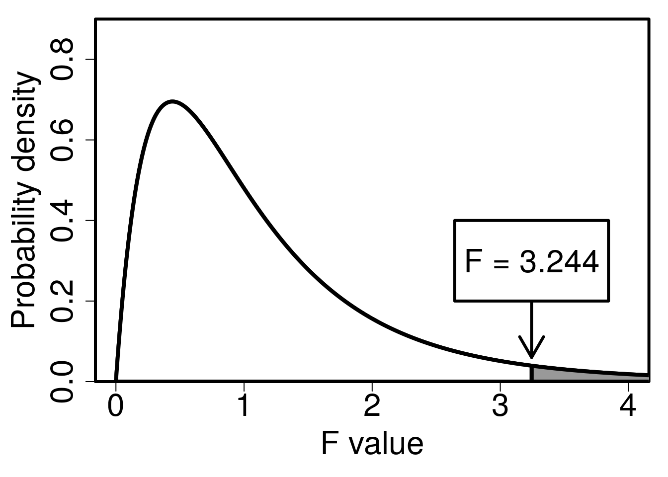
Figure 24.2: F-distribution with \(df = 4\) for the numerator and \(df = 15\) for the denominator. The arrow indicates an \(F\) value calculated from fig wasp species wing length measurements for five different species and four measurements per species. Fig wasp wing lengths were collected from a site near La Paz in Baja, Mexico 2010.

The area shaded in grey in Figure 24.2, where \(F\) > 3.2443976, is approximately \(P =\) 0.041762. This is our p-value. Since \(P < 0.05\), we can reject the null hypothesis that all mean species wing lengths are the same, because the variance among species wing lengths is significantly higher than the variance within species wing lengths. Note that the critical value of \(F\) (i.e., for which \(P = 0.05\)) is 3.0555683, so for any \(F\) value above this (for \(df1 = 5\) and \(df2 = 19\)), we would reject \(H_{0}\).

When running an ANOVA in a statistical program, output includes (at least) the calculated F-statistic, degrees of freedom, and the p-value. Figure 24.3 shows the one-way ANOVA output of the test of fig wasp wing lengths in jamovi.

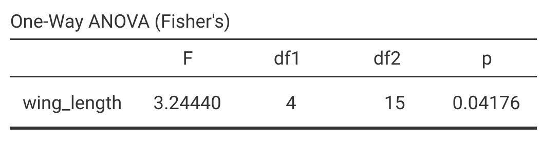
Figure 24.3: Jamovi output for a one-way ANOVA of wing length measurements in five species of fig wasps collected in 2010 near La Paz in Baja, Mexico.

Jamovi is quite minimalist for a one-way ANOVA (The jamovi project, 2024), but these four statistics (\(F\), \(df1\), \(df2\), and \(p\)) are all that is really needed. Most statistical programs will show ANOVA output that includes the \(SS\) and mean squares among (\(MS_{\mathrm{among}}\)) and within (\(MS_{\mathrm{within}}\)) groups.

Analysis of Variance Table

Response: wing_length
          Df  Sum Sq  Mean Sq F value  Pr(>F)  
Species    4 0.36519 0.091297  3.2444 0.04176 *
Residuals 15 0.42210 0.028140                  
---
Signif. codes:  0 '***' 0.001 '**' 0.01 '*' 0.05 '.' 0.1 ' ' 1

The above output, taken from R (R Core Team, 2022), includes the same information as jamovi (\(F\), \(df1\), \(df2\), and \(p\)), but also includes \(SS\) and mean variances. We can also get this information from jamovi if we want it (see Chapter 27).

24.3 Assumptions of ANOVA

As with the t-test (see Section 22.4), there are some important assumptions that we make when using an ANOVA. Violating these assumptions will mean that our Type I error rate (\(\alpha\)) is, again, potentially misleading. Assumptions of ANOVA include the following (Box et al., 1978; Sokal & Rohlf, 1995):

1. Observations are sampled randomly
2. Observations are independent of one another
3. Groups have the same variance
4. Errors are normally distributed

Assumption 1 just means that observations are not biased in any particular way. For example, if the fig wasps introduced at the start of this chapter were used because they were the largest wasps that were collected for each species, then this would violate the assumption that the wing lengths were sampled randomly from the population.

Assumption 2 means that observations are not related to one another in some confounding way. For example, if all of the Het1 wasps came from one fig tree, and all of the Het2 wasps came from a different fig tree, then wing length measurements are not really independent within species. In this case, we could not attribute differences in mean wing length to species. The differences could instead be attributable to wasps being sampled from different trees (more on this in Chapter 27).

Assumption 3 is fairly self-explanatory. The ANOVA assumes that all of the groups in the dataset (e.g., species in the case of the fig wasp wing measurements) have the same variance, that is, we assume homogeneity of variances (as opposed to heterogeneity of variances). In general, ANOVA is reasonably robust to deviations from homogeneity, especially if groups have similar sample sizes (Blanca et al., 2018). This means that the Type I error rate is about what we want it to be (usually \(\alpha = 0.05\)), even when the assumption of homogeneity of variances is violated. In other words, we are not rejecting the null hypothesis when it is true more frequently than we intend! We can test the assumption that group variances are the same using a Levene’s test in the same way that we did for the independent samples t-test in Chapter 23. If we reject the null hypothesis that groups have the same variance, then we should potentially consider a non-parametric alternative test such as the Kruskal-Wallis H test (see Chapter 26).

Assumption 4 is the equivalent of the t-test assumption from Section 22.4 that sample means are normally distributed around the true mean. What the assumption means is that if we were to repeatedly resample data from a population, the sample means that we calculate would be normally distributed. For the fig wasp wing measurements, this means that if we were to go back out and repeatedly collect four fig wasps from each of the five species, then sample means of species wing length and overall wing length would be normally distributed around the true means. Due to the central limit theorem (see Chapter 16), this assumption becomes less problematic with increasing sample size. We can test if the sample data are normally distributed using a Q-Q plot or Shapiro-Wilk test (the same procedure used for the t-test). Fortunately, the ANOVA is quite robust to deviations from normality (Schmider et al., 2010), but if data are not normally distributed, we should again consider a non-parametric alternative test such as the Kruskal-Wallis H test (see Chapter 26).

References

Blanca, M. J., Alarcón, R., Arnau, J., Bono, R., & Bendayan, R. (2018). Effect of variance ratio on ANOVA robustness: Might 1.5 be the limit? Behavior Research Methods, 50(3), 937–962. https://doi.org/10.3758/s13428-017-0918-2

Box, G. E. P., Hunter, W. G., & Hunter, S. J. (1978). Statistics for Experimenters: An Introduction to Design, Data Analysis, and Model Building. John Wiley & Sons, New York, USA.

Duthie, A. B., Abbott, K. C., & Nason, J. D. (2015). Trade-offs and coexistence in fluctuating environments: evidence for a key dispersal-fecundity trade-off in five nonpollinating fig wasps. American Naturalist, 186(1), 151–158. https://doi.org/10.1086/681621

Miller, I., & Miller, M. (2004). John E. Freund’s mathematical statistics (7th ed., p. 614). Pearson Prentice Hall, Upper Saddle River, New Jersey, USA.

R Core Team. (2022). R: A language and environment for statistical computing. R Foundation for Statistical Computing. https://www.R-project.org/

Schmider, E., Ziegler, M., Danay, E., Beyer, L., & Bühner, M. (2010). Is it really robust?: Reinvestigating the robustness of ANOVA against violations of the normal distribution assumption. Methodology, 6(4), 147–151. https://doi.org/10.1027/1614-2241/a000016

Sokal, R. R., & Rohlf, F. J. (1995). Biometry (3rd ed., p. 887). W. H. Freeman & Company, New York, USA.

The jamovi project. (2024). Jamovi (version 2.5). https://www.jamovi.org

---

54. Technically polynomially, but the distinction really is not important for understanding the concept. In general, the number of possible comparisons between groups is described by a binomial coefficient, \[\binom{g}{2} = \frac{g!}{2\left(g - 2 \right)!}.\] The number of combinations therefore increases with increasing group number (g).↩︎

55. To get the 0.4, we can first calculate the probability that we (correctly) do not reject \(H_{0}\) for all 10 pair-wise species combinations \((1 - 0.05)^{10} \approx 0.60\), then subtract from 1, \(P(Reject\:H_{0}) = 1 - (1 - 0.05)^{10} \approx 0.4\). That is, we find the probability of there not being a Type I error in the first test \((1 - 0.05)\), and the second test \((1 - 0.05)\), and so forth, thereby multiplying \((1 - 0.05)\) by itself 10 times. This gives the probability of not committing any Type I error across all 10 tests, so the probability that we commit at least one Type I error is 1 minus this probability.↩︎

56. The F-distribution was originally discovered in the context of the ratio of random variables with Chi-square distributions, with each variable being divided by its own degree of freedom (Miller & Miller, 2004). We will look at the Chi-square distribution in Chapter 29.↩︎

57. https://bradduthie.github.io/stats/app/f_distribution/↩︎

58. Note that the \(SS\) divided by the degrees of freedom (\(N - 1\)) is a variance. For technical reasons (Sokal & Rohlf, 1995), we cannot simply calculate the mean variance of groups (i.e., the mean of \(s^{2}_{\mathrm{Het1}}\), \(s^{2}_{\mathrm{Het2}}\), etc.). We need to sum up all the squared deviations from group means before dividing by the relevant degrees of freedom (i.e., dfs for the among and within group variation).↩︎

59. In this case, weighing by sample size is not so important because each species has the same number of samples. But when different groups have different numbers of samples, we need to multiply by sample number so that each group contributes proportionally to the SS.↩︎

60. Note that \(df_{\mathrm{among}} = 4\) and \(df_{\mathrm{within}} = 15\) sum to 19, which is the total df of the entire dataset (\(N - 1 = 20 - 1 = 19\)). This is always the case for the ANOVA; the overall df constrains the degrees of freedom among and within groups.↩︎