Chapter 29 Frequency and count data
In this book, we have introduced hypothesis testing as a tool to determine if variables were sampled from a population with a specific mean (one sample t-test in Section 22.1), or if different groups of variables were sampled from a population with the same mean (the independent samples t-test in Section 22.2 and ANOVA in Chapter 24). In these tests, the variables for which we calculated the means were always continuous (e.g., fig wasp wing lengths, nitrogen concentration in parts per million). That is, the dependent variables of the t-test and ANOVA could always, at least in theory, take any real value (i.e., any decimal). And the comparison was always between the means of categorical groups (e.g., fig wasp species or study sites). But not every variable that we measure will be continuous. For example, in Chapter 5, we also introduced discrete variables, which can only take discrete counts (1, 2, 3, 4, and so forth). Examples of such count data might include the number of species of birds in a forest or the number of days in the year for which an extreme temperature is recorded. Chapter 15 included some examples of count data when introducing probability distributions (e.g., counts of heads or tails in coin flips, or the number of people testing positive for COVID-19). Count data are discrete because they can only take integer values. For example, there cannot be 14.24 bird species in a forest; it needs to be a whole number.
In the biological and environmental sciences, we often want to test whether or not observed counts are significantly different from some expectation. For example, we might hypothesise that the probability of flowers being red versus blue in a particular field is the same. In other words, \(P(flower = red) = 0.5\) and \(P(flower = Blue) = 0.5\). By this logic, if we were to collect 100 flowers at random from the field, we would expect 50 to be red and 50 to be blue. If we actually went out and collected 100 flowers at random, but found 46 to be red and 54 to be blue, would this be sufficiently different from our expectation to reject the null hypothesis that the probability of sampling a red versus blue flower is the same? We could test this null hypothesis using a Chi-square goodness of fit test (Section 29.1). Similarly, we might want to test if two different count variables (e.g., flower colour and flower species) are associated with one another (e.g., if blue flowers are more common in one species than another species). We could test this kind of hypothesis using a Chi-square test of association.
Before introducing the Chi-square goodness of fit test or the Chi-square test of association, it makes sense to first introduce the Chi-square (\(\chi^{2}\)) distribution. The general motivation for introducing the Chi-square distribution is the same as it was for the t-distribution (Chapter 19) or F-distribution (Section 24.1). We need some probability density distribution that is our null distribution, which is what we predict if our null hypothesis is true. We then compare this null distribution to our test statistic to find the probability of sampling a test statistic as or more extreme if the null hypothesis is really true (i.e., a p-value).
29.1 Chi-square distribution
The Chi-square (\(\chi^{2}\)) distribution is a continuous distribution in which values of \(\chi^{2}\) can be any real number greater than or equal to 0. We can generate a \(\chi^{2}\) distribution by adding up squared values that are sampled from a standard normal distribution (Sokal & Rohlf, 1995), hence the ‘square’ in ‘Chi-square’. There is a lot to unpack in the previous sentence, so we can go through it step by step. First, we can take another look at the standard normal distribution from Section 15.4.4 (Figure 15.9). Suppose that we randomly sampled four values from the standard normal distribution.
- \(x_{1} = -1.244\)
- \(x_{2} = 0.162\)
- \(x_{3} = -2.214\)
- \(x_{4} = 2.071\)
We can square all of these values, then add up the squares,
\[\chi^{2} = (-1.244)^{2} + (0.162)^{2} + (-2.214)^{2} + (2.071)^{2}.\]
Note that \(\chi^{2}\) cannot be negative because when we square a number that is either positive or negative, we always end up with a positive value (e.g., \(-2^{2} = 4\), see Section 1.1). The final value is \(\chi^{2} = 10.76462\). Of course, this \(\chi^{2}\) value would have been different if our \(x_{i}\) values (\(x_{1}\), \(x_{2}\), \(x_{3}\), and \(x_{4}\)) had been different. And if we are sampling randomly from the normal distribution, we should not expect to get the same \(\chi^{2}\) value from four new random standard normal deviates. We can therefore ask: if we were to keep sampling four standard normal deviates and calculating new \(\chi^{2}\) values, what would be the distribution of these \(\chi^{2}\) values? The answer is shown in Figure 29.1.
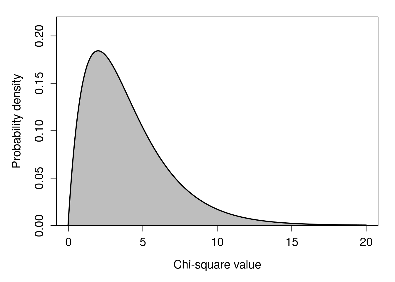
Figure 29.1: A Chi-square distribution that is the expected sum of four squared standard normal deviates, i.e., the sum of four values sampled from a standard normal distribution and squared.
Looking at the shape of Figure 29.1, we can see that most of the time, the sum of deviations from the mean of \(\mu = 0\) will be about 2. But sometimes we will get a much lower or higher value of \(\chi^{2}\) by chance, if we sample particularly low or high values of \(x_{i}\).
If we summed a different number of squared \(x_{i}\) values, then we would expect the distribution of \(\chi^{2}\) to change. Had we sampled fewer than four \(x_{i}\) values, the expected \(\chi^{2}\) would be lower just because we are adding up fewer numbers. Similarly, had we sampled more than four \(x_{i}\) values, the expected \(\chi^{2}\) would be higher just because we are adding up more numbers. The shape of the \(\chi^{2}\) distribution65 is therefore determined by the number of values sampled (\(n\)), or more specifically the degrees of freedom (\(df\), or sometimes \(v\)), which in a sample is \(df = n - 1\). This is the same idea as the t-distribution from Chapter 19, which also changed shape depending on the degrees of freedom. Figure 29.2 shows the different \(\chi^{2}\) probability density distributions for different degrees of freedom.
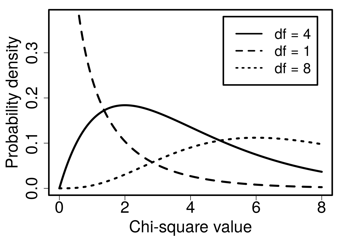
Figure 29.2: Probability density functions for three different Chi-square distributions, each of which has different degrees of freedom (\(df\)).
As with the F-distribution from Section 24.1, visualising the \(\chi^{2}\) distribution is easier using an interactive application66. And as with the F-distribution, it is not necessary to memorise how the \(\chi^{2}\) distribution changes with different degrees of freedom. The important point is that the distribution changes with different degrees of freedom, and we can map probabilities to the \(\chi^{2}\) value on the x-axis in the same way as any other distribution.
What does any of this have to do with count data? It actually is a bit messy. The \(\chi^{2}\) distribution is not a perfect tool for comparing observed and expected counts (Sokal & Rohlf, 1995). After all, counts are integer values, and the \(\chi^{2}\) distribution is clearly continuous (unlike, e.g., the binomial or Poisson distributions from Section 15.4). The \(\chi^{2}\) distribution is in fact a useful approximation for testing counts, and one that becomes less accurate when sample size (Slakter, 1968) or expected count size (Tate & Hyer, 1973) is small. Nevertheless, we can use the \(\chi^{2}\) distribution as a tool for testing whether observed counts are significantly different from expected counts. The first test that we will look at is the goodness of fit test.
29.2 Chi-square goodness of fit
The first kind of test that we will consider for count data is the goodness of fit test. In this test, we have some number of counts that we expect to observe (e.g., expected counts of red versus blue flowers), then compare this expectation to the counts that we actually observe. If the expected and observed counts differ by a lot, then we will get a large test statistic and reject the null hypothesis. A simple concrete example will make this a bit more clear.
Recall the practical in Chapter 17, in which players of the mobile app game ‘Power Up!’ chose a small, medium, or large dam at the start of the game. Suppose that we are interested in the size of dam that policy-makers choose to build when playing the game, so we find 60 such people in Scotland and ask them to play the game. Perhaps we do not think that the policy-makers will have any preference for a particular dam size (and therefore just pick one of the three dam sizes at random). We would therefore expect an equal number of small, medium, and large dams to be selected among the 60 players. That is, for our expected counts of each dam size (\(E_{\mathrm{size}}\)), we expect 20 small (\(E_{\mathrm{small}} = 20\)), 20 medium (\(E_{\mathrm{medium}} = 20\)), and 20 large (\(E_{\mathrm{large}} = 20\)) dams in total (because \(60/3 = 20\)).
Of course, even if our players have no preference for a particular dam size, the number of small, medium, and large dams will not always be exactly the same. The expected counts might still be a bit different from the observed counts of each dam size (\(O_{\mathrm{size}}\)). Suppose, for example, we find that out of our total 60 policy-makers, we observe 18 small (\(O_{\mathrm{small}} = 18\)), 24 medium (\(O_{\mathrm{medium}} = 24\)), and 18 large (\(O_{\mathrm{large}} = 18\)), dams were actually chosen by game players. What we want to test is the null hypothesis that there is no significant difference between expected and observed counts.
- \(H_{0}\): There is no significant difference between expected and observed counts.
- \(H_{A}\): There is a significant difference between expected and observed counts.
To get our test statistic67, we now just need to take each observed count, subtract the expected count, square this difference, divide by the expected count, then add everything up,
\[\chi^{2} = \frac{(18 - 20)^{2}}{20} + \frac{(24 - 20)^{2}}{20} + \frac{(18 - 20)^{2}}{20}.\]
We can calculate the values in the numerator. Note that all of these numbers must be positive (e.g., \(18 - 20 = -2\), but \(-2^{2} = 4\)),
\[\chi^{2} = \frac{4}{20} + \frac{16}{20} + \frac{4}{20}.\]
When we sum the three terms, we get a value of \(\chi^{2} = 1.2\). Note that if all of our observed values had been the same as the expected values (i.e., 20 small, medium, and large dams actually chosen), then we would get a \(\chi^{2}\) value of 0. The more the observed values differ from the expectation of 20, the higher the \(\chi^{2}\) will be. We can now check to see if the test statistic \(\chi^{2} = 1.2\) is sufficiently large to reject the null hypothesis that our policy-makers have no preference for small, medium, or large dams. There are \(n = 3\) categories of counts (small, medium, and large), meaning that there are \(df = 3 - 1 = 2\) degrees of freedom. As it turns out, if the null hypothesis is true, then the probability of observing a value of \(\chi^{2} = 1.2\) or higher (i.e., the p-value) is \(P = 0.5488\). Figure 29.3 shows the appropriate \(\chi^{2}\) distribution plotted, with the area above the test statistic \(\chi^{2} = 1.2\) shaded in grey.
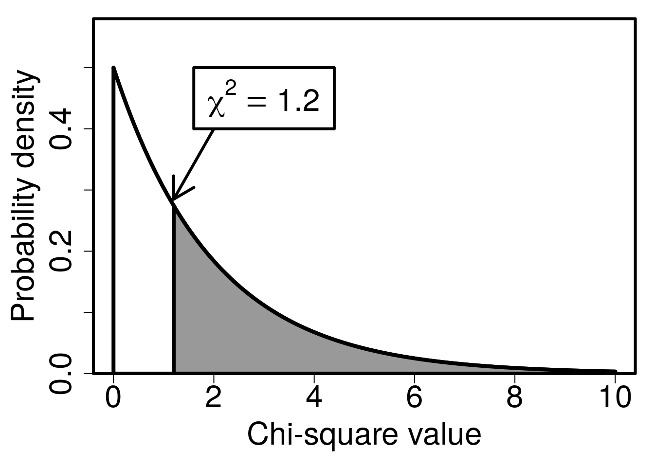
Figure 29.3: A Chi-square distribution with 2 degrees of freedom, used in a goodness of fit test to determine if all players of the mobile game ‘Power Up!’ have the same preference for initial dam size. An arrow indicates a \(\chi^{2}\) value of 1.2 on the x-axis, and grey shading indicates the probability of a more extreme value under the null hypothesis.
Because \(P > 0.05\), we do not reject the null hypothesis that there is no significant difference between expected and observed counts of chosen dam sizes.
Note that this was a simple example. For a goodness of fit test, we can have any number of different count categories (at least, any number greater than 1). The expectations also do not need to be integers. For example, if we only managed to find 59 policy makers instead of 60, then our expected counts would have been \(59/3 = 19.33\) instead of \(60/3 = 20\). The expectations also do not need to be the same. For example, we could have tested the null hypothesis that twice as many policy-makers would choose large dams (i.e., \(E_{\mathrm{large}} = 40\), \(E_{\mathrm{medium}} = 10\), and \(E_{\mathrm{small}} = 10\)). For \(n\) categories, the more general equation for the \(\chi^{2}\) statistic is,
\[\chi^{2} = \sum_{i = 1}^{n} \frac{\left(O_{i} - E_{i}\right)^{2}}{E_{i}}.\]
We can therefore use this general equation to calculate a \(\chi^{2}\) for any number of categories (\(n\)). Next, we will look at testing associations between counts in different types of categories.
29.3 Chi-square test of association
The second kind of test that we will consider for count data is the Chi-square test of association. While the goodness of fit test focused on a single categorical variable (dam sizes in the example above), the Chi-square test of association focuses on two different categorical variables. What we want to know is whether or not the two categorical variables are independent of one another (Box et al., 1978). In other words, does knowing something about one variable tell us anything about the other variable? A concrete example will make it easier to explain. We can again make use of the Chapter 17 game ‘Power Up!’. As mentioned in the previous section, game players choose a small, medium, or large dam at the start of the game. Players can play the game on either an Android or macOS mobile device. We therefore have two categorical variables: dam size and OS type. We might want to know, do Android users choose the same dam sizes as macOS users? In other words, are dam size and OS type associated? We can state this as a null and alternative hypothesis.
- \(H_{0}\): There is no association between OS and dam size choice.
- \(H_{A}\): There is an association between OS and dam size choice.
Consider the data in Table 29.1, which show counts of Android versus macOS users and their dam choices.
| Small | Medium | Large | |
|---|---|---|---|
| Android | 8 | 16 | 6 |
| macOS | 10 | 8 | 12 |
Just looking at the counts in Table 29.1, it appears that there might be an association between the two variables. For example, Android users appear to be more likely to choose a medium dam than macOS users. Medium dams are the most popular choice for Android users, but they are the least popular choice for macOS users. Nevertheless, could this just be due to chance? If it were due to chance, then how unlikely are the counts in Table 29.1? In other words, if Android and macOS users in the whole population really do choose dam sizes at the same frequencies, then what is the probability of getting a sample of 60 players in which the choices are as or more unbalanced as this? This is what we want to answer with our Chi-square test of association.
The general idea is the same as with the Chi-square goodness of fit test. We have our observed values (Table 29.1). We now need to find the expected values to calculate a \(\chi^{2}\) value. But the expected values are now a bit more complicated. With the goodness of fit test in Section 29.2, we just assumed that all categories were equally likely (i.e., the probability of choosing each size dam was the same). There were 60 players and three dam sizes, so the expected frequency of each dam choice was 60/3 = 20. Now it is different. We are not testing if dam sizes or OS choices are the same. We want to know if they are associated with one another. That is, regardless of the popularity of Android versus macOS, or the frequency with which small, medium and large dams are selected, do Android users choose different dam sizes than macOS users? If dam size is not associated with OS, then we would predict that the relative frequency of small, medium, and large dams would be the same for both Android and macOS.
To find the expected counts of each variable combination (e.g., Android and Small, or macOS and Large), we need to get the probability that each category is selected independently. For example, what is the probability of a player selecting a large dam, regardless of the OS that they are using? Table 29.2 shows these probabilities as additional rows and columns added onto Table 29.1
| Small | Medium | Large | Probability | |
|---|---|---|---|---|
| Android | 8 | 16 | 6 | 0.5 |
| macOS | 10 | 8 | 12 | 0.5 |
| Probability | 0.3 | 0.4 | 0.3 | – |
Since there are 30 total Android users (\(8 + 16 + 6 = 30\)) and 30 total macOS users (\(10 + 8 + 12 = 30\)), the probability of a player having an Android OS is \(30/60 = 0.5\), and the probability of a player having a macOS is also \(30 / 60 = 0.5\). Similarly, there are 18 small, 24 medium, and 18 large dam choices in total. Hence, the probability of a player choosing a small dam is \(18/60 = 0.3\), medium is \(24/60 = 0.4\), and large is \(18/60 = 0.3\). If these probabilities combine independently68, then we can multiply them to find the probability of a particular combination of categories. For example, the probability of a player using Android is 0.5 and choosing a small dam is 0.3, so the probability of a player having both Android and a small dam is \(0.5 \times 0.3 = 0.15\) (see Chapter 16 for an introduction to probability models). The probability of a player using Android and choosing a medium dam is \(0.5 \times 0.4 = 0.2\). We can fill in all of these joint probabilities in a new Table 29.3.
| Small | Medium | Large | Probability | |
|---|---|---|---|---|
| Android | 0.15 | 0.2 | 0.15 | 0.5 |
| macOS | 0.15 | 0.2 | 0.15 | 0.5 |
| Probability | 0.3 | 0.4 | 0.3 | – |
From Table 29.3, we now have the probability of each combination of variables. Note that all of these probabilities sum to 1.
\[0.15 + 0.2 + 0.15 + 0.15 + 0.2 + 0.15 = 1.\]
To get the expected count of each combination, we just need to multiply the probability by the sample size, i.e., the total number of players (\(N = 60\)). For example, the expected count of players who use Android and choose a small dam will be \(0.15 \times 60 = 9\). Table 29.4 fills in all of the expected counts. Note that the sum of all the counts equals our sample size of 60.
| Small | Medium | Large | Sum | |
|---|---|---|---|---|
| Android | 9 | 12 | 9 | 30 |
| macOS | 9 | 12 | 9 | 30 |
| Sum | 18 | 24 | 18 | – |
We now have both the observed (Table 29.2) and expected (Table 29.4) counts (remember that the expected counts do not need to be integers). To get our \(\chi^{2}\) test statistic, we use the same formula as in Section 29.2,
\[\chi^{2} = \sum_{i = 1}^{n} \frac{\left(O_{i} - E_{i}\right)^{2}}{E_{i}}.\]
There are six total combinations of OS and dam size, so there are \(n = 6\) values to sum up,
\[\chi^{2} = \frac{(8-9)^2}{9} + \frac{(16 - 12)^{2}}{12} + ... + \frac{(16 - 12)^{2}}{12} + \frac{(8-9)^2}{9}.\]
If we sum all of the six terms, we get a value of \(\chi^{2} = 4.889\). We can compare this to the null \(\chi^{2}\) distribution as we did in the Section 29.2 goodness of fit test, but we need to know the correct degrees of freedom. The correct degrees of freedom69 is the number of categories in variable 1 (\(n_{1}\)) minus 1, times the number of categories in variable 2 (\(n_{2}\)) minus 1,
\[df = (n_{1} - 1) \times (n_{2} - 1).\]
In our example, the degrees of freedom equals the number of dam types minus 1 (\(n_{\mathrm{dam}} = 3 - 1)\) times the number of operating systems minus 1 (\(n_{\mathrm{OS}} = 2 - 1\)). The correct degrees of freedom is therefore \(df = 2 \times 1 = 2\). We now just need to find the p-value for a Chi-square distribution with two degrees of freedom and a test statistic of \(\chi^{2} = 4.889\). We get a value of about \(P = 0.0868\). In other words, if \(H_{0}\) is true, then the probability of getting a \(\chi^{2}\) of 4.889 or higher is \(P = 0.0868\). Consequently, because \(P > 0.05\), we would not reject the null hypothesis. We should therefore conclude that there is no evidence for an association between OS and dam size choice.
Jamovi will calculate the \(\chi^{2}\) value and get the p-value for the appropriate degrees of freedom (The jamovi project, 2024). To do this, it is necessary to input the categorical data (e.g., Android, macOS) in a tidy format, which will be a focus of Chapter 31.
There is one final point regarding expected and observed values of the Chi-square test of association. There is another way of getting these expected values that is a bit faster (and more widely taught) but does not demonstrate the logic of expected counts as clearly. If we wanted to, we could sum the rows and columns of our original observations. Table 29.5 shows the original observations with the sum of each row and column.
| Small | Medium | Large | Sum | |
|---|---|---|---|---|
| Android | 8 | 16 | 6 | 30 |
| macOS | 10 | 8 | 12 | 30 |
| Sum | 18 | 24 | 18 | – |
We can get the expected counts from Table 29.5 if we multiply each row sum by each column sum, then divide by the total sample size (\(N = 60\)). For example, to get the expected counts of Android users who choose a small dam, we can multiply \((18 \times 30)/60 = 9\). To get the expected counts of macOS users who choose a medium dam, we can multiply \((30 \times 24)/60 = 12\). This works for all of combinations of rows and columns, so we could do it to find all of the expected counts from Table 29.4.
References
A random variable \(X\) has a \(\chi^{2}\) distribution if and only if its probability density function is defined by (Miller & Miller, 2004), \[f(x) = \left\{\begin{array}{ll}\frac{1}{2^{\frac{2}{v}}\Gamma\left(\frac{v}{2}\right)}x^{\frac{v-2}{2}}e^{-\frac{x}{2}} & \quad for\:x > 0 \\ 0 & \quad elsewhere \end{array}\right.\] In this equation, \(v\) is the degrees of freedom of the distribution.↩︎
A lot of statisticians will use \(X^{2}\) to represent the test statistic here instead of \(\chi^{2}\) (Sokal & Rohlf, 1995). The difference is the upper case ‘X’ versus the Greek letter Chi, ‘\(\chi\)’. The X is used since the test statistic we calculate here is not technically from the \(\chi^{2}\) distribution, just an approximation. We will not worry about the distinction here, and to avoid confusion, we will just go with \(\chi^{2}\).↩︎
We can call these the ‘marginal probabilities’.↩︎
This formula works due to a bit of a mathematical trick (Sokal & Rohlf, 1995). The actual logic of the degrees of freedom is a bit more involved. From our total of \(k = 6\) different combinations, we actually need to subtract one degree of freedom for the total sample size (\(N = 60\)), then a degree of freedom for each variable probability estimated (i.e., subtract \(n_{1} - 1\) and \(n_{2} - 1\) because we need this many degrees of freedom to get the \(n_{1}\) and \(n_{2}\) probabilities, respectively; if we have all but one probability, then we know the last probability because the probabilities must sum to 1). Since we lose \(n_{1} - 1\) and \(n_{2} - 1\) degrees of freedom, and 1 for the sample size, this results in \(df = k - (n_{1} - 1) - (n_{2} - 1) - 1\). In the case of the ‘Power Up!’ example, we get \(df = 6 - (3 - 1) - (2 - 1) - 1 = 2\). The \(df = (n_{1} - 1) \times (n_{2} - 1)\) formulation is possible because \(k = n_{1} \times n_{2}\) (Sokal & Rohlf, 1995).↩︎