Chapter 2 Data organisation
In the field or the lab, data collection can be messy. Often data need to be recorded with a pencil and paper, and in a format that is easiest for writing in adverse weather or a tightly controlled laboratory. Sometimes data from a particular sample, such as a bird nest (Figure 2.1), cannot all be collected in one place.
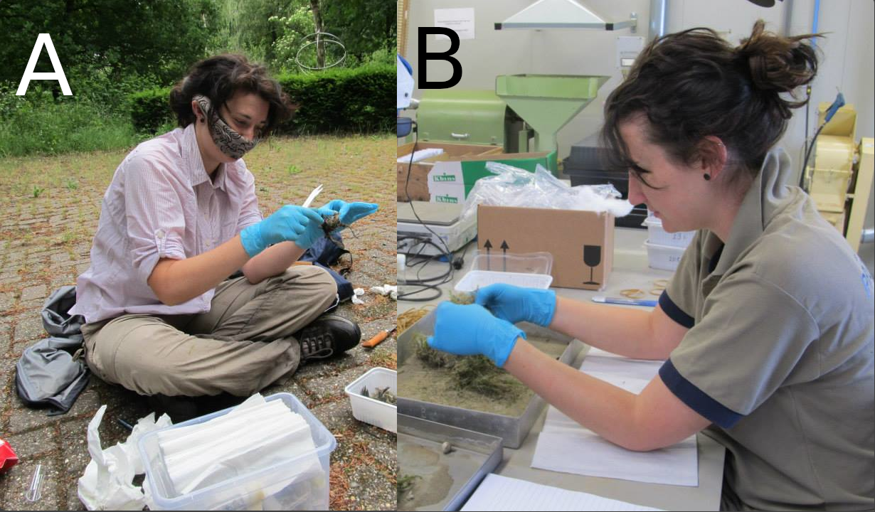
Figure 2.1: Dr Becky Boulton collects data from nest boxes in the field (A), then she processes nest material in the lab (B).
Data are sometimes missing due to circumstances outwith the researcher’s control, and data are usually not collected in a format that is immediately ready for statistical analysis. Consequently, we often need to reorganise data from a lab or field book to a spreadsheet on the computer. Fortunately, there are some generally agreed upon guidelines for formatting data for statistical analysis. This chapter introduces the tidy format (Wickham, 2014), which is widely used for structuring data files. This chapter will provide an example of how to put data into a tidy format, and how to save a dataset into a file that can be read and used in jamovi (The jamovi project, 2024).
2.1 Tidy data
After data are collected, they need to be stored digitally (i.e., in a computer file, such as a spreadsheet). This should happen as soon as possible so that back-up copies of the data can be made. Retaining field and lab notes as a record of the originally collected data is also a good idea. Sometimes it is necessary to return to these notes, even years after data collection. Often we will want to double-check to make sure that we copied a value or observation correctly from handwritten notes to a spreadsheet. Note that sometimes data can be input directly into a spreadsheet or mobile application, bypassing handwritten notes altogether, but it is usually helpful to have a physical copy of collected data.
Most biological and environmental scientists store data digitally in the form of a spreadsheet. Spreadsheets enable data input, manipulation, and calculation in a highly flexible way. Most spreadsheet programs even have some capacity for data visualisation and statistical analysis. For the purposes of statistical analysis, spreadsheets are probably most often used for inputting data in a way that can be used by more powerful statistical software. Commonly used spreadsheet programs are MS Excel, Google Sheets, and LibreOffice Calc. The interface and functions of these programs are very similar, nearly identical for most purposes. They can all open and save the same file types (e.g., XLSX, ODS, CSV), and they all have the same overall look, feel, and functionality for data input, so the program used is mostly a matter of personal preference. In this book, we will use LibreOffice because it is completely free and open source, and easily available to download (http://libreoffice.org). Excel and Google Sheets are also completely fine to use.
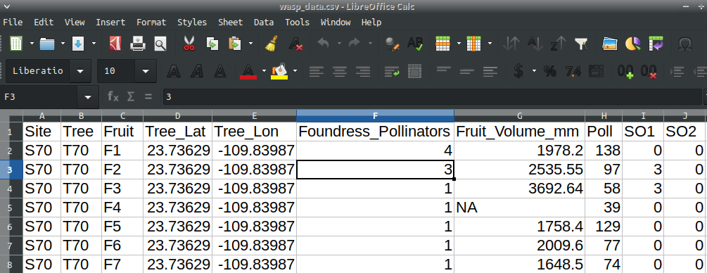
Figure 2.2: LibreOffice spreadsheet showing data from fig fruits collected in 2010. Each row is a unique sample (fruit), and columns record properties of the fruit.
Spreadsheets are separated into individual rectangular cells, which are identified by a specific column and row (Figure 2.2). Columns are indicated by letters, and rows are indicated by numbers. We can refer to a specific cell by its letter and number combination. For example, the active cell in Figure 2.2 is F3, which has a value of ‘3’ indicating the value recorded in that specific measurement (in this case, foundress pollinators in a fig fruit). We will look more at how to interact with the spreadsheet in Chapter 3, but for now we will focus on how the data are organised.
There are a lot of potential ways that data could be organised in a spreadsheet. For good statistical analysis, there are a few principles that are helpful to follow. Whenever we collect data, we record observations about different units. For example, we might make one or more measurements on a tree, a patch of land, or in a sample of soil. In this case, trees, land patches, or soil samples are our units of observation. Each attribute of a unit that we are measuring is a variable. These variables might include tree heights and leaf lengths, forest cover in a patch of land, or carbon and nitrogen content of a soil sample. Tidy datasets that can be used in statistical analysis programs are defined by three characteristics (Wickham, 2014):
- Each variable gets its own column.
- Each observation gets its own row.
- Different units of observation require different data files.
If, for example, we were to measure the heights and leaf lengths for 4 trees, we might organise the data as in Table 2.1.
| Tree | Species | Height (m) | Leaf Length (cm) |
|---|---|---|---|
| 1 | Oak | 20.3 | 8.1 |
| 2 | Oak | 25.4 | 9.4 |
| 3 | Maple | 18.2 | 12.5 |
| 4 | Maple | 16.7 | 11.3 |
By convention (Wickham, 2014), variables tend to be in the left-most columns if they are known in advance or fixed in some way by the data collection or experiment (e.g., tree number or species in Table 2.1). In contrast, variables that are actually measured tend to be in the right-most columns (e.g., tree height or leaf length). This is more for readability of the data; jamovi will not care about the order of data columns.
2.2 Data files
Data can be saved using many different file types. File type is typically indicated by an extension following the name of a file and a full stop. For example, ‘photo.png’ would indicate a PNG image file named ‘photo’. A peer-reviewed journal article might be saved as a PDF, e.g., ‘Wickham2014.pdf’. A file’s type affects what programs can be used to open it. One relevant distinction to make is between text files and binary files.
Text files are generally very simple. They only allow information to be stored as plain text; no colour, bold, italic, or anything else is encoded. All of the information is just made up of characters on one or more lines. This sounds so simple as to be almost obsolete; what is the point of not allowing anything besides plain text? The point is that text files are generally much more secure for long-term storage. The plain text format makes data easier to recover if a file is corrupted, is readable by a wider range of software, and is more amenable to version control (version control is a tool that essentially saves the whole history of a folder, and potentially different versions of it in parallel; it is not necessary for introductory statistics but is often critical for big collaborative projects). There are many types of text files with extensions such as TXT, CSV, HTML, R, CPP, or MD. For data storage, we will use comma-separated value (CSV) files. As the name implies, CSV files include plain text separated by commas. Each line of the CSV file is a new row, and commas separate information into columns. These CSV files can be opened in any text editor, but they are also recognised by nearly all spreadsheet programs and statistical software. The data shown in Figure 2.2 are from a CSV file called ‘wasp_data.csv’. Figure 2.3 shows the same data when opened with a text editor.
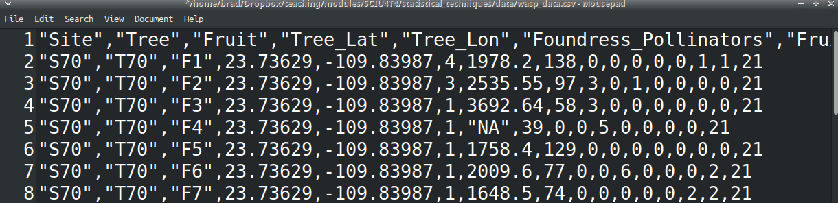
Figure 2.3: Plain text comma-separated value (CSV) file showing data from fig fruits collected in 2010. Each line is a unique row and unit of observation (fruit), and commas separate the data into columns in which the variables of fruit are recorded. The file has been opened in a program called ‘Mousepad’, but it could also be opened in any text editor such as gedit, Notepad, vim, or emacs. It could also be opened in spreadsheet programs such as LibreOffice Calc, MS Excel, or Google Sheets, or in any number of statistical programs.
The data shown in Figure 2.3 are not easy to read or work with, but the format is highly effective for storage because all of the information is in plain text. The information will therefore always look exactly the same, and it can be easily recovered by any text editor, even after years pass and old software inevitably becomes obsolete.
Binary files are different from text files and contain information besides just plain text. This information could include formatted text (e.g., bold, italic), images, sound, or video (basically, anything that can be stored in a file). The advantages of being able to store this kind of information are obvious, but the downside is that the information needs to be interpreted in a specific way, usually using a specific program. Examples of binary files include those with extensions such as DOC, XLS, PNG, GIF, MP3, or PPT. Some file types such as DOCX are not technically binary files, but a collection of zipped files (which, in the case of DOCX, include plain text files). Overall, the important point is that saving data in a text file format such as CSV is generally more secure.
2.3 Managing data files
Managing data files (or any files) effectively requires some understanding of how files are organised on a computer or cloud storage. In mobile phone applications, file organisation is often hidden, so it is not obvious where a file actually goes when it is saved on a device. Many people find files in these applications using a search function. The ability to search for files like this, or at least the tendency to do so regularly, is actually a relatively new phenomenon. And it is an approach to file organisation that does not work quite as well on non-mobile devices (i.e., anything that is not a phone or tablet), especially for big projects. On laptop and desktop computers, it is really important to know where files are being saved, and to ideally have an organisational system that makes it easy to find specific files without having to use a search tool.
On a computer, files are stored in a series of nested folders. You can think of the storage space on a computer, cloud, or network drive, as a big box. The big box can contain other smaller boxes (folders, in this analogy), or it can contain items that you need (files, in this analogy). Figure 2.4 shows the general idea. On this computer, there is a folder called ‘brad’, which has inside it five other folders (Figure 2.4A). Each of the five inner folders is used to store more folders and files for a specific class from 2006. Clicking on the ‘Biostatistics’ folder leads to the sub-folders inside it, and to files saved specifically for a biostatistics class (e.g., homework assignments, lecture notes, and an exam review document). Files on a computer therefore have a location that we can find using a particular path. We can write the path name using slashes to indicate nested folders. For example, the file ‘HW9.scx’ in Figure 2.4B would have the path name ‘/home/brad/Spring_2006/Biostatistics/HW9.scx’. Each folder is contained within slashes, and the file name itself is after the last slash.
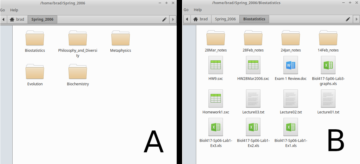
Figure 2.4: File directory of a computer showing (A) the file organisation of classes taken during spring 2006. Within one folder (B), there are multiple sub-folders and files associated with a biostatistics class.
These path names might look slightly different depending on the computer operating system that you are using. But the general idea of files nested within folders is the same. Figure 2.5 shows the same folder ‘Spring_2006’ saved in a different location, on OneDrive.
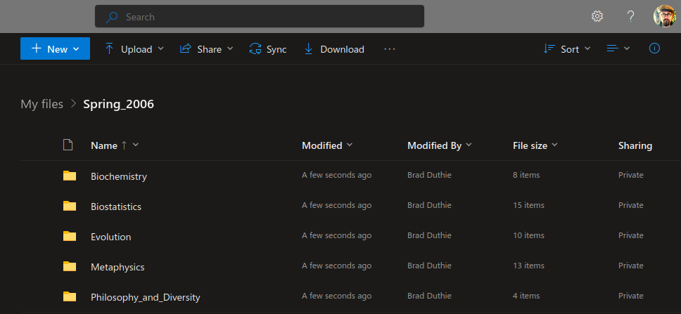
Figure 2.5: OneDrive file directory showing the file organisation of classes taken during spring 2006.
The path style ‘/home/user/folder/file.txt’ is used for Linux and macOS. Windows has the same general file organisation (Figure 2.6). Path names for storing files on the hard drive of a Windows computer look something like ‘C:\Users\MyName\Desktop\Spring_2006\Biostatistics\HW9.scx’. The ‘C:\’ is the root directory of the hard drive; it is called ‘C’ for historical reasons (‘A:\’ and ‘B:\’ used to be for floppy disks; the ‘A:\’ floppy disks had about 1.44 MB of storage, and ‘B:\’ had even less, so these are basically obsolete).
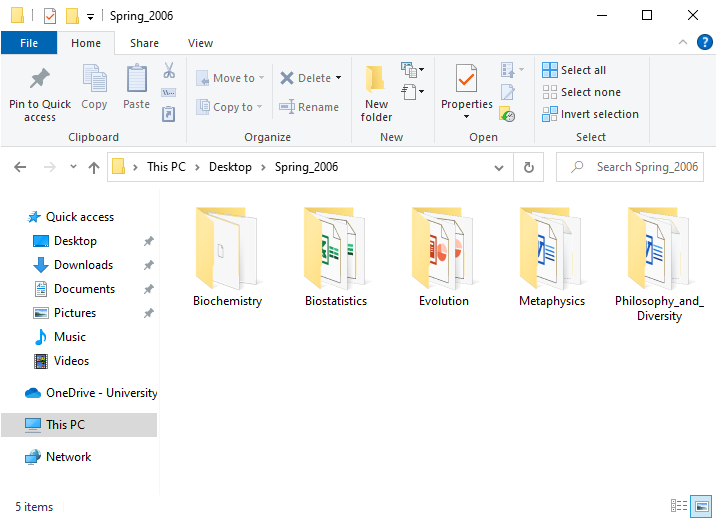
Figure 2.6: Windows file directory showing the file organisation of classes taken during spring 2006. In this case, the ‘Spring_2006’ folder is located on the desktop; the path to the folder is visible in the toolbar above the folders.
The details are not as important as the idea of organising files in a logical way that allows you to know roughly where to find important files on a computer or cloud drive. It is usually a good idea to give every unique project or subject (e.g., university class, student group, holiday plans, health records) its own folder. This makes it much easier to find related files such as datasets, lecture notes, or assignments when necessary. It is usually possible to right-click somewhere in a directory to create a new folder. In Figure 2.6, there is even a ‘New folder’ button in the toolbar with a yellow folder icon above it. It takes some time to organise files this way, and to get used to saving files in specific locations, but it is well worth it in the long-term.