Chapter 20 Practical. z- and t-intervals
This chapter focuses on applying the concepts from Chapter 18 and Chapter 19 in jamovi (The jamovi project, 2024). Specifically, we will practice calculating confidence intervals (CIs). There will be four exercises focused on calculating CIs in jamovi. To complete the first two exercises, you will need the distrACTION module in jamovi. If you need to download it again, the instructions to do this are in the second exercise of Chapter 17 (briefly, go to the Modules option and select ‘jamovi library’, then scroll down until you find the ‘distraACTION’ module).
The data for this chapter are inspired by ongoing work in the Woodland Creation and Ecological Networks (WrEN) project (Fuentes-Montemayor, Park, et al., 2022; Fuentes-Montemayor, Watts, et al., 2022). The WrEN project is led by a collaboration between University of Stirling researchers Dr Elisa Fuentes-Montemayor and Prof Kirsty Park, and at Forest Research, Prof Kevin Watts (https://www.wren-project.com/). It focuses on questions about what kinds of conservation actions should be prioritised to restore degraded ecological networks. The WrEN project encompasses a huge amount of work and data collection from hundreds of surveyed secondary or ancient woodland sites. Here we will focus on observations of tree diameter at breast height (DBH) and grazing to calculate confidence intervals.
20.1 Confidence intervals with distrACTION
First, it is important to download the distrACTION module if it has not been downloaded already. If the distrACTION module has already been downloaded (see Chapter 17), it should appear in the toolbar of jamovi. Once the distrACTION module has been made available, download the WrEN trees dataset38 and open it in a spreadsheet. Notice that the dataset is not in a tidy format. There are four different sites represented by different columns in the dataset. The numbers under each column are measurements of tree diameter at breast height (DBH) in centimetres. Before doing anything else, it is therefore necessary to put the WrEN dataset into a tidy format. The tidy dataset should include two columns: one for site and the other for DBH.
Once the WrEN trees dataset has been reorganised into a tidy format, save it as a CSV file and open it in jamovi. In jamovi, go to Exploration and Descriptives in the toolbar and build a histogram that shows the distribution of DBH. Do these data appear to be roughly normal? Why or why not?
Next, calculate the grand mean and standard deviation of tree DBH (i.e., the mean and standard deviation of trees across all sites).
Grand mean: _____________________
Grand standard deviation: _____________________
We will use this mean and standard deviation to compute quantiles and obtain 95% z-scores. First, click on the distrACTION icon in the toolbar. From the distrACTION pull-down menu, select ‘Normal Distribution’. To the left, you should see boxes to input parameter values for the mean and standard deviation (SD). Below the ‘Parameters’ options, you should also see different functions for computing probability or quantiles. To the right, you should see a standard normal distribution (i.e., a normal distribution with a mean of 0 and a standard deviation of 1).
For this exercise, we will assume that the population of DBH from which our sample came is normally distributed. In other words, if we somehow had access to all possible DBH measurements in the woodland sites (not just the 120 trees sampled), we assume that DBH would be normally distributed. To find the probability of sampling a tree within a given interval of DBH (e.g., greater than 30), we therefore need to build this distribution with the correct mean and standard deviation. We do not know the true mean (\(\mu\)) and standard deviation (\(\sigma\)) of the population, but our best estimate of these values are the mean (\(\bar{x}\)) and standard deviation (\(s\)) of the sample, as reported above (i.e., the grand mean and standard deviation). Using the Mean and SD parameter input boxes in distrACTION, we can build a normal distribution with the same mean and standard deviation as our sample. Do this now by inputting the calculated Grand mean and Grand standard deviation from above in the appropriate boxes. Note that the normal distribution on the right has the same shape, but the table of parameters has been updated to reflect the mean and standard deviation.
In Chapter 17, we calculated the probability of sampling a value within a given interval of the normal distribution. If we wanted to do the same exercise here, we might find the probability of sampling a DBH < 30 using the Compute probability function (the answer is p = 0.264). Instead, we are now going to do the opposite using the Compute quantile(s) function. We might want to know, for example, what 75% of DBH values will be less than (i.e., what is the cutoff DBH, below which DBH values will be lower than this cutoff with a probability of 0.75). To find this, uncheck the ‘Compute probability’ box and check the ‘Compute quantile(s)’ box. Make sure that the ‘cumulative quantile’ radio button is selected, then set p = 0.75 (Figure 20.1).
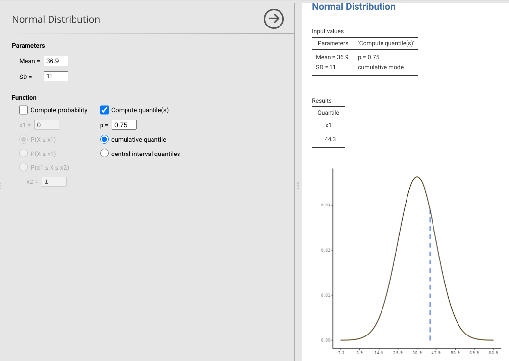
Figure 20.1: Jamovi interface for the ‘distrACTION’ module, in which quantiles have been computed to find the diameter at breast height (DBH) below which 75% of DBHs will be given a normal distribution with a mean of 36.9 and standard deviation of 11. Data for these parameter values were inspired by the Woodland Creation and Ecological Networks (WrEN) project.
From Figure 20.1, we can see that the cumulative 0.75 quantile is 44.3, so if DBH is normally distributed with the mean and standard deviation calculated above, 75% of DBH values in a population will be below 44.3 cm. Using the same principles, what is the cumulative 0.4 quantile for the DBH data?
Quantile: _____________________
We can also use the Compute quantile(s) option in jamovi to compute interval quantiles. For example, if we want to know the DBH values within which 95% of the probability density is contained, we can set p = 0.95, then select the radio button ‘central interval quantiles’. Do this for the DBH data. From the Results table on the right, what interval of DBH values will contain 95% of the probability density around the mean?
Interval: _____________________
Remember that we are looking at the full sample distribution of DBH. That is, getting intervals for the probability of sampling DBH values around the mean, not confidence intervals around the mean as introduced in Chapter 18. How would we get confidence intervals around the mean? That is, what if we want to say that we have 95% confidence that the mean lies between two values? We would need to use the standard deviation of the sample mean \(\bar{x}\) around the true mean \(\mu\), rather than the sample standard deviation. Recall from Section 12.6 that the standard error is the standard deviation of \(\bar{x}\) values around \(\mu\). We can therefore use the standard error to calculate confidence intervals (CIs) around the mean value of DBH. From the ‘Descriptives’ panel in jamovi (recall that this is under the ‘Exploration’ button), find the standard error of DBH,
Std. error of Mean: ___________________
Now, go back to the distrACTION Normal Distribution and put the DBH mean into the parameters box as before. But this time, put the standard error calculated above into the box for SD. Next, choose the ‘Compute quantile(s)’ option and set p = 0.95 to calculate a 95% confidence interval. Based on the Results table, what can you infer are the lower and upper 95% CIs around the mean?
Lower 95% CI: ________________
Upper 95% CI: ________________
Remember that this assumed that the sample means (\(\bar{x}\)) are normally distributed around the true mean (\(\mu\)). But as we saw in Chapter 19, when we assume that our sample standard deviation (\(s\)) is the same as the population standard deviation (\(\sigma\)), then the shape of the normal distribution will be at least a bit off. Instead, we can get a more accurate estimate of CIs using a t-distribution. Jamovi usually does this automatically when calculating CIs outside of the distrACTION module. To get 95% CIs, go back to the Descriptives panel in jamovi, then choose DBH as a variable. Scroll down to the Statistics options and check ‘Confidence interval for Mean’ under the Mean Dispersion options, and make sure that the number in the box is 95 for 95% confidence. Confidence intervals will appear in the Descriptives table on the right. From this Descriptives table now, write the lower and upper 95% CIs below.
Lower 95% CI: ________________
Upper 95% CI: ________________
You might have been expecting a bit more of a difference, but remember, for sufficiently large sample sizes (around N = 30), the normal and t-distributions are very similar (see Chapter 19). We really do not expect much of a difference until sample sizes become small, which we will see in Exercise 20.3.
20.2 Confidence intervals from z- and t-scores
While jamovi can be very useful for calculating CIs from a dataset, you might also need to calculate CIs from just a set of summary statistics (e.g., mean, standard error, and sample size). This activity will demonstrate how to calculate CIs from z- and t-scores. Recall the formula for lower and upper CIs from Section 18.1,
\[LCI = \bar{x} - (z \times SE),\]
\[UCI = \bar{x} + (z \times SE).\]
We could calculate 95% CIs for DBH with just the sample mean (\(\bar{x}\)), z-score (\(z\)), and standard error (SE). We have already calculated \(\bar{x}\) and SE for the DBH in Exercise 20.1 above, so we just need to figure out z. Recall that z-scores are standard normal deviates, that is, deviations from the mean given a standard normal distribution, in which the mean equals 0 and standard deviation equals 1. For example, \(z = -1\) is 1 standard deviation below the mean of a standard normal distribution, and \(z = 2\) is 2 standard deviations above the mean of a standard normal distribution. What values of z contain 95% of the probability density of a standard normal distribution? We can use the distrACTION module again to find this out. Select ‘Normal Distribution’ from the pull-down menu of the distrACTION module. Notice that by default, a standard normal distribution is already set (Mean = 0 and SD = 1). All that we need to do now is compute quantiles for p = 0.95. From these quantiles, what is the proper z-score to use in the equations for LCI and UCI above?
z-score: ________________
Now, use the values of \(\bar{x}\), \(z\), and SE for DBH in the equations above to calculate lower and upper 95% CIs again.
Lower 95% CI: ________________
Upper 95% CI: ________________
Are these CIs the same as what you calculated in Exercise 20.1?
Lastly, instead of using the z-score, we can do the same with a t-score. We can find the appropriate t-score from the t-distribution in the distrACTION module. To get the t-score, click on the distrACTION module button and choose ‘T-Distribution’ from the pull-down menu. To get quantiles with the t-distribution, we need to know the degrees of freedom (\(df\)) of the sample. Chapter 19 explains how to calculate \(df\) from the sample size \(N\). What are the appropriate \(df\) for DBH?
\(df\): _________________
Put the df in the Parameters box. Ignore the box for lambda (\(\lambda\)); this is not needed. Under the Function options, choose ‘Compute quantile(s)’ as before to calculate Quantiles. From the Results table, what is the proper t-score to use in the equations for LCI and UCI?
t-score: _______________
Again, use the values of \(\bar{x}\), \(t\), and \(SE\) for DBH in the equations above to calculate lower and upper 95% CIs.
Lower 95% CI: ________________
Upper 95% CI: ________________
How similar are the estimates for lower and upper CIs when using z- versus t-scores. Reflect on any similarities or differences that you see in all of these different ways of calculating CIs.
20.3 Confidence intervals for different sample sizes
In Exercises 20.1 and 20.2, the sample size of DBH was fairly large (\(N = 120\)). Now, we will calculate CIs for the mean DBH of each of the four different sites using both z- and t-scores. These sites have much different sample sizes. From the Descriptives tool in jamovi, write the sample sizes for DBH split by site below.
Site 1182: \(N =\) _________
Site 1223: \(N =\) _________
Site 3008: \(N =\) _________
Site 10922: \(N =\) _________
For which of these sites would you predict CIs calculated from z-scores versus t-scores to differ the most?
Site: ______________
The next part of this exercise is self-guided. In Exercises 20.1 and 20.2, you used different approaches for calculating 95% CIs from the normal and t-distributions. Now, fill in Table 20.1 reporting 95% CIs calculated using each distribution from the four sites using any method you prefer.
| Site | N | 95% CIs (Normal) | 95% CIs (t-distribution) |
|---|---|---|---|
| 1182 | |||
| 1223 | |||
| 3008 | |||
| 10922 |
Next, do the same in Table 20.2, but now calculate 99% CIs instead of 95% CIs.
| Site | N | 99% CIs (Normal) | 99% CIs (t-distribution) |
|---|---|---|---|
| 1182 | |||
| 1223 | |||
| 3008 | |||
| 10922 |
What do you notice about the difference between CIs calculated from the normal distribution versus the t-distribution across the different sites?
In your own words, what do these CIs actually mean?
We will now move on to calculating CIs for proportions.
20.4 Proportion confidence intervals
We will now try calculating CIs for proportional data using the WrEN Sites dataset39.
Notice that there are more sites included than there were in the dataset used in Exercises 20.1–20.3, and that some of these sites are grazed while others are not (column ‘Grazing’). From the Descriptives options, find the number of sites grazed versus not grazed (hint, remember from Chapter 17 to put ‘Grazing’ in the variable box and click the ‘Frequency tables’ checkbox).
Grazed: ____________
Not Grazed: _____________
From these counts above, what is the estimate (\(p\), or more technically \(\hat{p}\), with the hat indicating that it is an estimate) of the proportion of sites that are grazed?
\(p =\) __________
Chapter 18 explained how to calculate lower and upper CIs for binomial distributions (i.e., proportion data). It showed how to calculate Wald CIs, but also noted that Clopper-Pearson CIs are generally more accurate. First, we will calculate Wald CIs by hand, then use jamovi to calculate Clopper-Pearson CIs. To calculate the Wald CIs, we can use equations similar to the ones used for LCI and UCI from Exercise 20.2 above,
\[LCI = p - z \times \mathrm{SE}(p),\]
\[UCI = p + z \times \mathrm{SE}(p),\]
We have already calculated \(p\), and we can find z-scores for CIs in the same way that we did in Exercise 20.2 (i.e., the z-scores associated with 95% CIs do not change just because we are working with proportions). All that is left to calculate LCI and UCI are the standard errors of the proportions. Remember from Chapter 18 that these are calculated differently from a standard error of continuous values such as diameter breast height. The formula for standard error of a proportion is,
\[\mathrm{SE}(p) = \sqrt{\frac{p\left(1 - p\right)}{N}}.\]
We can estimate \(p\) as the total number of grazed sites divided by \(N\), where \(N\) is the total sample size. Using the above equation, what is the standard error of p?
SE(p) = ____________
Using this standard error, what are the Wald lower and upper 95% CIs around \(p\)?
Wald \(LCI_{95\%} =\) ______________
Wald \(UCI_{95\%} =\) ______________
Next, find the lower and upper 99% CIs around \(p\) and report them below (hint: the only difference here from the calculation of the 95% CIs is the z-score).
Wald \(LCI_{99\%} =\) ______________
Wald \(UCI_{99\%} =\) ______________
Do you notice anything unusual about the lower 99% CI?
Now we can use jamovi to find the Clopper-Pearson 95 and 99% CIs. Jamovi does this for us, so no calculation is required. To calculate Clopper-Pearson CIs, Find the ‘Frequencies’ button on the toolbar in the ‘Analyses’ tab. Click on ‘Frequencies’, then choose ‘2 Outcomes’ from the pull-down menu. You will see a box on the left called ‘Proportion Test (2 Outcomes)’. From here, move ‘Grazing’ from the left box to the right box. Under Additional Statistics, check the box for ‘Confidence intervals’, and make sure that the interval is 95. A table called ‘Proportion Test (2 Outcomes)’ will appear to the right. Find the row with the Grazing Level ‘Yes’, then report what you see for \(p\), and the lower and upper CIs below.
\(p =\) __________
Clopper-Pearson \(LCI_{95\%} =\) ______________
Clopper-Pearson \(UCI_{95\%} =\) ______________
To calculate 99% CIs, change the number in the Interval box from 95 to 99. Report the 99% CIs below.
Clopper-Pearson \(LCI_{99\%} =\) ______________
Clopper-Pearson \(UCI_{99\%} =\) ______________
What do you notice about the difference between the Wald CIs and the Clopper-Pearson CIs?
20.5 Another proportion confidence interval
Next, find the 80, 95, and 99% CIs for the proportion of sites that are classified as Ancient woodland using the Clopper-Pearson method for calculating binomial CIs. First consider an 80% CI.
\(LCI_{80\%} =\) ______________
\(UCI_{80\%} =\) ______________
Next, calculate 95% CIs for the proportion of sites classified as Ancient woodland.
\(LCI_{95\%} =\) ______________
\(UCI_{95\%} =\) ______________
Finally, calculate 99% CIs for the proportion of sites classified as Ancient woodland.
\(LCI_{99\%} =\) ______________
\(UCI_{99\%} =\) ______________
Reflect again on what these values actually mean. For example, what does it mean to have 95% confidence that the proportion of sites classified as Ancient woodland are between two values? Are there any situations in which this might be useful, from a scientific or conservation standpoint? There is no right or wrong answer here, but CIs are very challenging to understand conceptually, so having now done the calculations to get them, it is a good idea to think again about what they mean.