Chapter 15 Introduction to probability models
Suppose that we flip a fair coin over a flat surface. There are two possibilities for how the coin lands on the surface. Either the coin lands on one side (heads) or the other side (tails), but we do not know the outcome in advance. If these two events (heads or tails) are equally likely, then we could reason that there is a 50% chance that a flipped coin will land heads up and a 50% chance that it will land heads down. What do we actually mean when we say this? For example, when we say that there is a 50% chance of the coin landing heads up, are we making a claim about our own uncertainty, how coins work, or how the world works? We might mean that we simply do not know whether or not the coin will land heads up, so a 50-50 chance just reflects our own ignorance about what will actually happen when the coin is flipped. Alternatively, we might reason that if a fair coin were to be flipped many times, all else being equal, then about half of flips should end heads up, so a 50% chance is a reasonable prediction for what will happen in any given flip. Or, perhaps we reason that events such as coin flips really are guided by chance on some deeper fundamental level, such that our 50% chance reflects some real causal metaphysical process in the world. These are questions concerning the philosophy of probability. The philosophy of probability is an interesting sub-discipline in its own right, with implications that can and do affect how researchers do statistics (Edwards, 1972; Gelman & Shalizi, 2013; Mayo, 1996; Mayo, 2021; Navarro & Foxcroft, 2022; Suárez, 2020).
In this chapter, we will not worry about the philosophy of probability16 and instead focus on the mathematical rules of probability as applied to statistics. These rules are important for predicting real-world events in the biological and environmental sciences. For example, we might need to make predictions concerning the risk of disease spreading in a population, or the risk of extreme events such as droughts occurring given increasing global temperatures. Probability is also important for testing scientific hypotheses. For example, if we sample two different groups and calculate that they have different means (e.g., two different fields have different mean soil nitrogen concentrations), we might want to know the probability that this difference between means could have arisen by chance. Here I will introduce practical examples of probability, then introduce some common probability distributions.
15.1 Instructive example
Probability focuses on the outcomes of trials, such as the outcome (heads or tails) of the trial of a coin flip. The probability of a specific outcome is the relative number of times it is expected to happen given a large number of trials,
\[P(outcome) = \frac{\mathrm{Number\:of\:times\:outcome\:occurs}}{\mathrm{Total\:number\:of\:trials}}.\]
For the outcome of a flipped coin landing on heads,
\[P(heads) = \frac{\mathrm{Flips\:landing\:on\:heads}}{\mathrm{Total\:number\:of\:flips}}.\]
As the total number of flips becomes very large, the number of flips that land on heads should get closer and closer to half the total, \(1/2\) or \(0.5\) (more on this later). The above equations use the notation \(P(E)\) to define the probability (\(P\)) of some event (\(E\)) happening. Note that the number of times an outcome occurs cannot be less than 0, so \(P(E) \geq 0\) must always be true. Similarly, the number of times an outcome occurs cannot be greater than the number of trials; the most frequently it can happen is in every trial, in which case the top and bottom of the fraction are the same value. Hence, \(P(E) \leq 1\) must also always be true. Probabilities therefore range from 0 (an outcome never happens) to 1 (an outcome always happens).
It might be more familiar and intuitive at first to think in terms of percentages (i.e., from 0 to 100% chance of an outcome, rather than from 0 to 1), but there are good mathematical reasons for thinking about probability on a 0–1 scale (it makes calculations easier). For example, suppose we have two coins, and we want to calculate the probability that they will both land on heads if we flip them at the same time. That is, we want to know the probability that coin 1 lands on heads and coin 2 lands on heads. We can assume that the coins do not affect each other in any way, so each coin flip is independent of the other (i.e., the outcome of coin 1 does not affect the outcome of coin 2, and vice versa – this kind of assumption is often very important in statistics). Each coin, by itself, is expected to land on heads with a probability of 0.5, \(P(heads) = 0.5\). When we want to know the probability that two or more independent events will happen, we multiply their probabilities. In the case of both coins landing on heads, the probability is therefore,
\[P(Coin_{1} = heads\:\cap\:Coin_{2} = heads) = 0.5 \times 0.5 = 0.25.\]
Note that the symbol \(\cap\) is basically just a fancy way of writing ‘and’ (technically, the intersection between sets; see set theory for details). Verbally, all this is saying is that the probability of coin 1 landing on heads and the probability of coin 2 landing on heads equals 0.5 times 0.5, which is 0.25.
But why are we multiplying to get the joint probability of both coins landing on heads? Why not add, for example? We could just take it as a given that multiplication is the correct operation to use when calculating the probability that multiple events will occur. Or we could do a simple experiment to confirm that 0.25 really is about right (e.g., by flipping two coins 100 times and recording how many times both coins land on heads). But neither of these options would likely be particularly satisfying. Let us first recognise that adding the probabilities cannot be the correct answer. If the probability of each coin landing on heads is 0.5, then adding probabilities would imply that the probability of both landing on heads is 0.5 + 0.5 = 1. This does not make any sense because we know that there are other possibilities, such as both coins landing on tails, or one coin landing on heads and the other landing on tails. Adding probabilities cannot be the answer, but why multiply?
We can think about probabilities visually, as a kind of probability space. When we have only one trial, then we can express the probability of an event along a line (Figure 15.1).
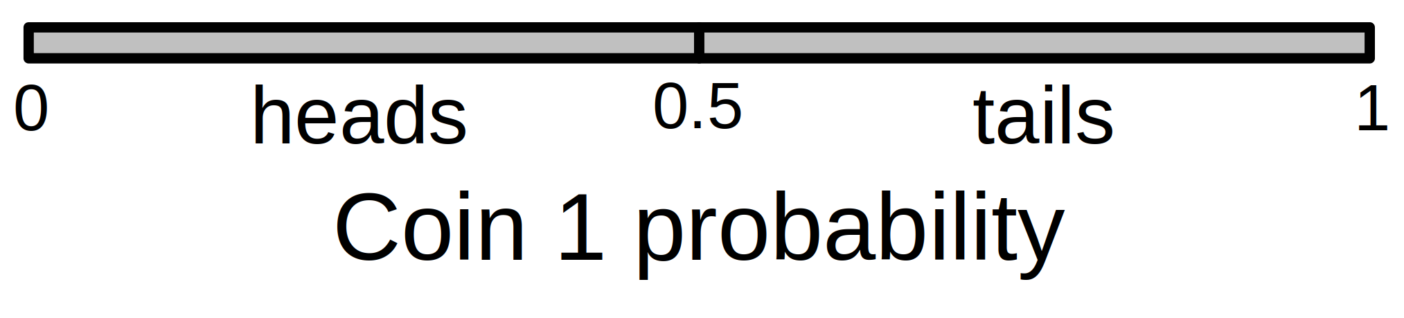
Figure 15.1: Total probability space for flipping a single coin and observing its outcome (heads or tails). Given a fair coin, the probability of heads equals a proportion 0.5 of the total probability space, while the probability of tails equals the remaining 0.5 proportion.
The total probability space is 1, and ‘heads’ occupies a density of 0.5 of the total space. The remaining space, also 0.5, is allocated to ‘tails’. When we add a second independent trial, we now need two dimensions of probability space (Figure 15.2). The probability of heads or tails for coin 1 (the horizontal axis of Figure 15.2) remains unchanged, but we add another axis (vertical this time) to think about the equivalent probability space of coin 2.
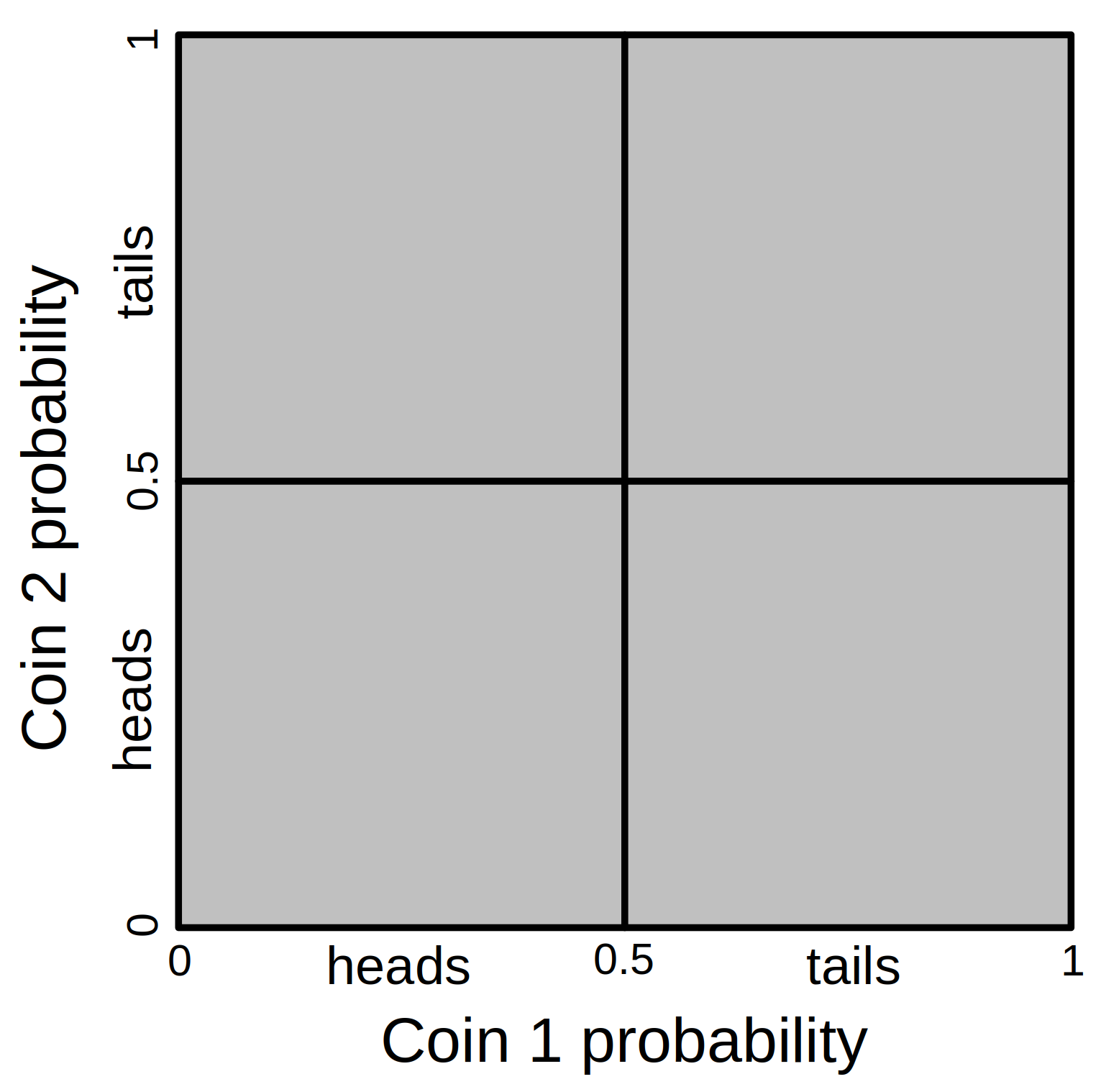
Figure 15.2: Total probability space for flipping two coins and observing their different possible outcomes (heads-heads, heads-tails, tails-heads, and tails-tails). Given two fair coins, the probability of flipping heads for each equals 0.25, which corresponds to the lower left square of the probability space.
Now we can see that the area in which both coin 1 and coin 2 land on heads has a proportion of 0.25 of the total area. This is a geometric representation of what we did when calculating \(P(Coin_{1} = heads\:\cap Coin_{2} = heads) = 0.5 \times 0.5 = 0.25.\) The multiplication works because multiplying probabilities carves out more specific regions of probability space. Note that the same pattern would apply if we flipped a third coin. In this case, the probability of all three coins landing on heads would be \(0.5 \times 0.5 \times 0.5 = 0.125\), or \(0.5^{3} = 0.125\).
What about when we want to know the probability of one outcome or another outcome happening? Here is where we add. Note that the probability of a coin flip landing on heads or tails must be 1 (there are only two possibilities!). What about the probability of both coins landing on the same outcome, that is, either both coins landing on heads or both landing on tails? We know that the probability of both coins landing on heads is \(0.25\). The probability of both coins landing on tails is also \(0.25\), so the probability that both coins land on either heads or tails is \(0.25 + 0.25 = 0.5\). The visual representation in Figure 15.2 works for this example too. Note that heads-heads and tails-tails outcomes are represented by the lower left and upper right areas of probability space, respectively. This is 0.5 (i.e., 50%) of the total probability space.
15.2 Biological applications
Coin flips are instructive, but the relevance for biological and environmental sciences might not be immediately clear. In fact, probability is extremely relevant in nearly all areas of the natural sciences. The following are just two hypothetical examples where the calculations in the previous section might be usefully applied:
From a recent report online, suppose you learn that 1 in 40 people in your local area is testing positive for COVID-19. You find yourself in a small shop with 6 other people. What is the probability that at least 1 of these 6 other people would test positive for COVID-19? To calculate this, note that the probability that any given person has COVID-19 is \(1/40 = 0.025\), which means that the probability that a person does not must be \(1 - 0.025 = 0.975\) (they either do or do not, and the probabilities must sum to 1). The probability that all 6 people do not have COVID-19 is therefore \((0.975)^6 = 0.859\). Consequently, the probability that at least 1 of the 6 people does have COVID-19 is \(1 - 0.859 = 0.141\), or \(14.1\%\).
Imagine you are studying a population of sexually reproducing, diploid (i.e., 2 sets of chromosomes), animals, and you find that a particular genetic locus has 3 alleles with frequencies \(P(A_{1}) = 0.40\), \(P(A_{2}) = 0.45\), and \(P(A_{3}) = 0.15\). What is the probability that a randomly sampled animal will be heterozygous with 1 copy of the \(A_{1}\) allele and 1 copy of the \(A_{3}\) allele? Note that there are 2 ways for \(A_{1}\) and \(A_{3}\) to arise in an individual, just like there were 2 ways to get a heads and tails coin in the Section 14.1 example (see Figure 14.2). The individual could either get an \(A_{1}\) in the first position and \(A_{3}\) in the second position, or an \(A_{3}\) in the first position and \(A_{1}\) in the second position. We can therefore calculate the probability as, \(P(A_{1}) \times P(A_{3}) + P(A_{3}) \times P(A_{1})\), which is \((0.40 \times 0.15) + (0.15 \times 0.4) = 0.12\), or 12% (in population genetics, we might use the notation \(p = P(A_{1})\) and \(r = P(A_{3})\), then note that \(2pr = 0.12\)).
In both of these examples, we made some assumptions, which might or might not be problematic. In the first example, we assumed that the 6 people in our shop were a random and independent sample from the local area (i.e., people with COVID-19 are not more or less likely to be in the shop, and the 6 people in the shop were not associated in a way that would affect their individual probabilities of having COVID-19). In the second example, we assumed that individuals mate randomly, and that there is no mutation, migration, or selection on genotypes (Hardy, 1908). It is important to recognise these assumptions when we are making them, because violations of assumptions could affect the probabilities of events!
15.3 Sampling with and without replacement
It is often important to make a distinction between sampling with or without replacement. Sampling with replacement just means that whatever has been sampled once gets put back into the population before sampling again. Sampling without replacement means that whatever has been sampled does not get put back into the population before sampling again. An example makes the distinction between sampling with and without replacement clearer.
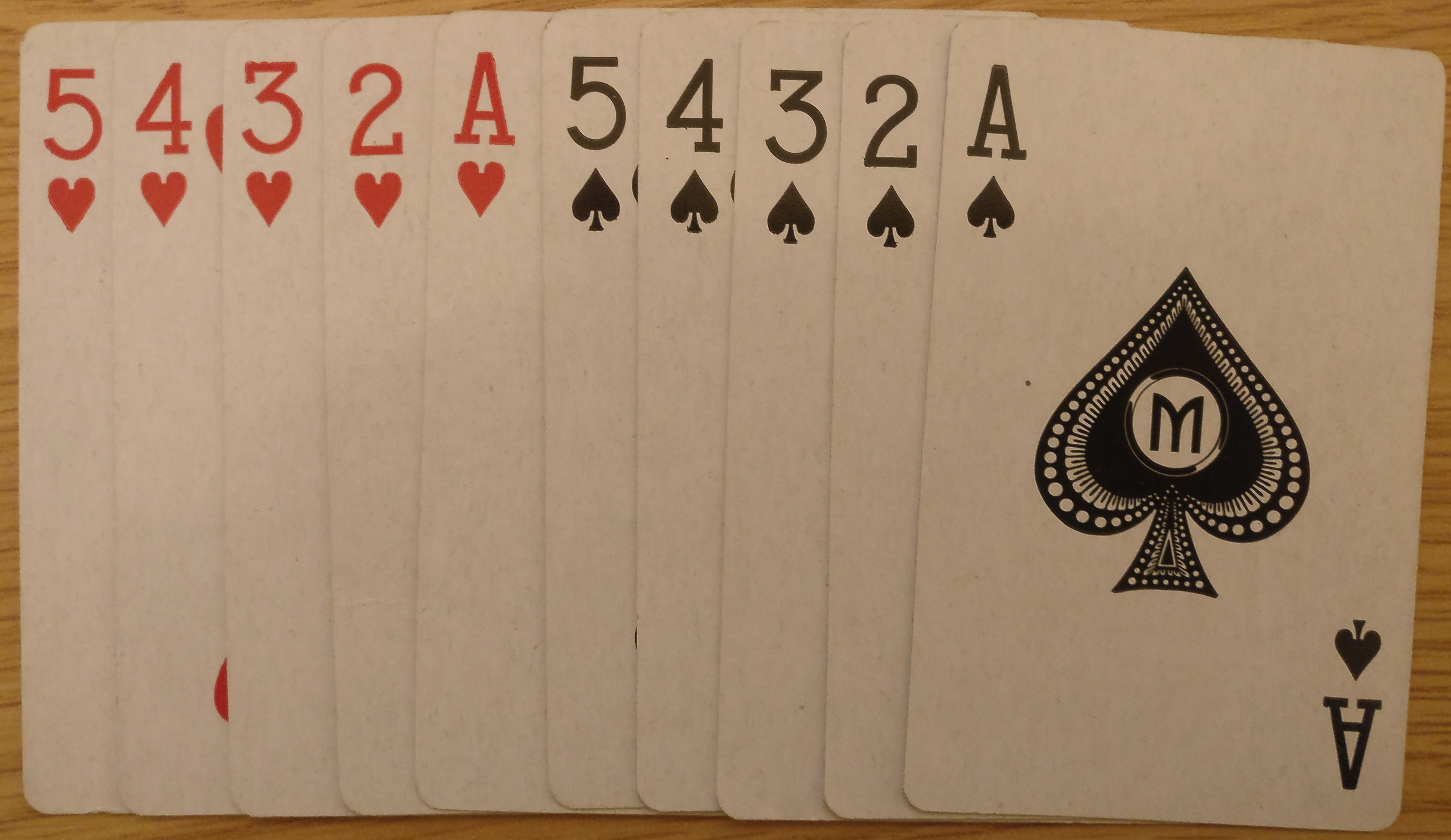
Figure 15.3: Playing cards can be useful for illustrating concepts in probability. Here we have 5 hearts (left) and 5 spades (right).
Figure 15.3 shows 10 playing cards: 5 hearts and 5 spades. If we shuffle these cards thoroughly and randomly select 1 card, what is the probability of selecting a heart? This is simply,
\[P(heart) = \frac{5\:\mathrm{hearts}}{10\mathrm{\:total\:cards}} = 0.5.\]
What is the probability of randomly selecting 2 hearts? This depends if we are sampling with or without replacement. If we sample 1 card, then put it back into the deck before sampling the second card, then the probability of sampling a heart does not change (in both samples, we have 5 hearts and 10 cards). Hence, the probability of sampling 2 hearts with replacement is \(P(heart) \times P(heart) = 0.5 \times 0.5 = 0.25\). If we do not put the first card back into the deck before sampling again, then we have changed the total number of cards. After sampling the first heart, we have one fewer heart in the deck and one fewer card, so the new probability for sampling a heart becomes,
\[P(heart) = \frac{4\:\mathrm{hearts}}{9\:\mathrm{total\:cards}} = 0.444.\]
Since the probability has changed after the first heart is sampled, we need to use this adjusted probability when sampling without replacement. In this case, the probability of sampling two hearts is \(0.5 \times 0.444 = 0.222\). This is a bit lower than the probability of sampling with replacement because we have decreased the number of hearts that can be sampled. When sampling from a set, it is important to consider whether the sampling is done with or without replacement.
15.4 Probability distributions
Up until this point, we have been considering the probabilities of specific outcomes. That is, we have considered the probability that a coin flip will be heads, that an animal will have a particular combination of alleles, or that we will randomly select a particular suit of card from a deck. Here we will move from specific outcomes and consider the distribution of outcomes. For example, instead of finding the probability that a flipped coin lands on heads, we might want to consider the distribution of the number of times that it does (in this case, 0 times or 1 time; Figure 15.4).
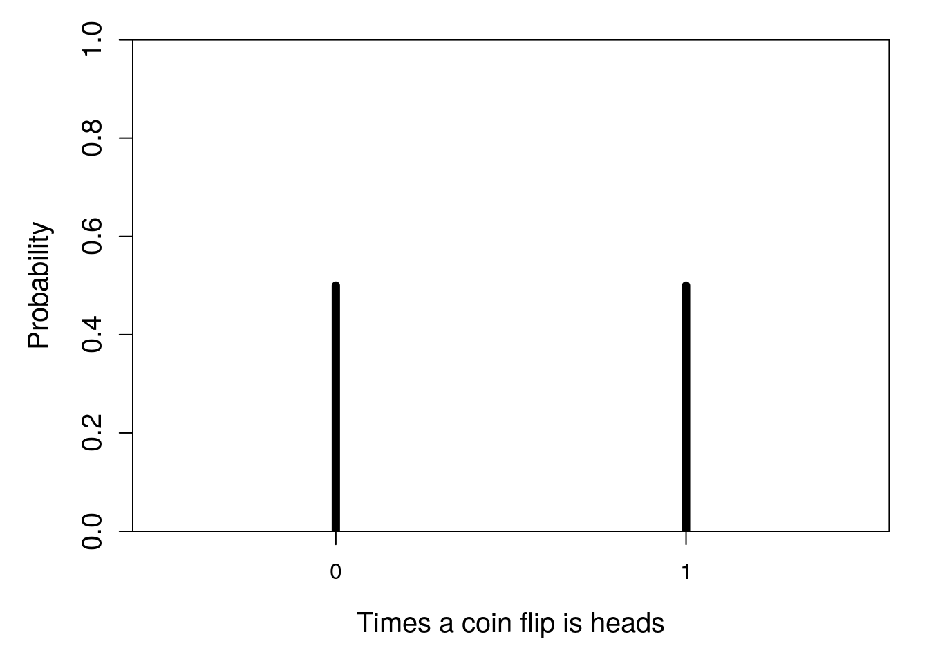
Figure 15.4: Probability distribution for the number of times that a flipped coin lands on heads in one trial.
This is an extremely simple distribution. There are only two discrete possibilities for the number of times the coin will land on heads, 0 or 1. And the probability of both outcomes is 0.5, so the bars in Figure 15.4 are the same height. Next, we will consider some more interesting distributions.
15.4.1 Binomial distribution
The simple distribution with a single trial of a coin flip was actually an example of a binomial distribution. More generally, a binomial distribution describes the number of successes in some number of trials (Miller & Miller, 2004). The word ‘success’ should not be taken too literally here; it does not necessarily indicate a good outcome, or an accomplishment of some kind. A success in the context of a binomial distribution just means that an outcome did happen as opposed to it not happening. If we define a coin flip landing on heads as a success, we could consider the probability distribution of the number of successes over 10 trials (Figure 15.5).
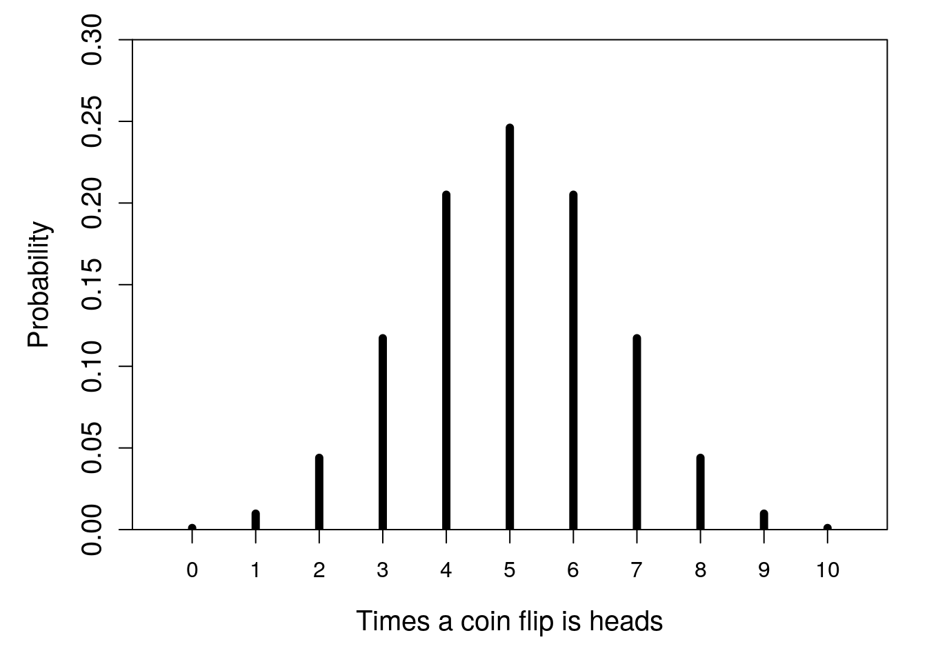
Figure 15.5: Probability distribution for the number of times that a flipped coin lands on heads in 10 trials.
Figure 15.5 shows that the most probable outcome is that 5 of the 10 coins flipped will land on heads. This makes some sense because the probability that any one flip lands on heads is 0.5, and 5 is 1/2 of 10. But 5 out of 10 heads happens only with a probability of about 0.25. There is also about a 0.2 probability that the outcome is 4 heads, and the same probability that the outcome is 6 heads. Hence, the probability that we get an outcome of between 4 and 6 heads is about \(0.25 + 0.2 + 0.2 = 0.65\). In contrast, the probability of getting all heads is very low (about 0.00098).
More generally, we can define the number of successes using the random variable \(X\). We can then use the notation \(P(X = 5) = 0.25\) to indicate the probability of 5 successes, or \(P(4 \leq X \leq 6) = 0.65\) as the probability that the number of successes is greater than or equal to 4 and less than or equal to 6.
Imagine that you were told a coin was fair, then flipped it 10 times. Imagine that 9 flips out of the 10 came up heads. Given the probability distribution shown in Figure 15.5, the probability of getting 9 or more heads in 10 flips given a fair coin is very low (\(P(X \geq 9) \approx 0.011\)). Would you still believe that the coin is fair after these 10 trials? How many, or how few, heads would it take to convince you that the coin was not fair? This question gets to the heart of a lot of hypothesis-testing in statistics, and we will see it more in Chapter 21.
Note that a binomial distribution does not need to involve a fair coin with equal probability of success and failure. We can consider again the first example in Section 15.2, in which 1 in 40 people in an area are testing positive for COVID-19, then ask what the probability is that 0–6 people in a small shop would test positive (Figure 15.6).
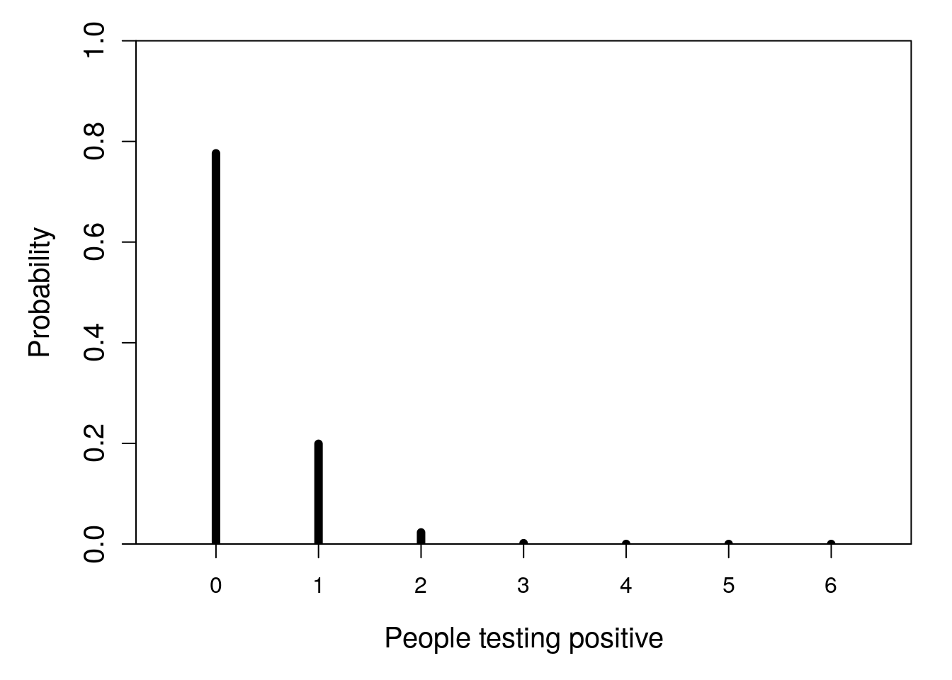
Figure 15.6: Probability distribution for the number of people who have COVID-19 in a shop of 6 when the probability of testing positive is 0.025.
Note that the shape of this binomial distribution is different from the coin flipping trials in Figure 15.5. The distribution is skewed, with a high probability of 0 successes and a diminishing probability of 1 or more successes.
The shape of a statistical probability distribution can be defined mathematically. Depending on the details (more on this later), we call the equation defining the distribution either a probability mass function or a probability density function. This book is about statistical techniques, not statistical theory, so we will relegate these equations to footnotes.17 What is important to know is that the shape of a distribution is modulated by parameters. The shape of a binomial distribution is determined by two parameters: the number of trials (\(n\)) and the probability of success (\(\theta\)). In Figure 15.5, there were 10 trials each with a success probability of 0.5 (i.e., \(n = 10\) and \(\theta = 0.5\)). In Figure 15.6, there were 6 trials each with a success probability of 0.025 (i.e., \(n = 6\) and \(\theta = 0.025\)). This difference in parameter values is why the two probability distributions have a different shape.
15.4.2 Poisson distribution
Imagine sitting outside on a park bench along a path that is a popular route for runners. On this particular day, runners pass by the bench at a steady rate of about 4 per minute, on average. We might then want to know the distribution of the number of runners passing by per minute. That is, given that we see 4 runners per minute on average, what is the probability that we will see just 2 runners pass in any given minute. What is the probability that we will see 8 runners pass in a minute? This hypothetical example is modelled with a Poisson distribution. A Poisson distribution describes events happening over some interval (e.g., happening over time or space). There are a lot of situations where a Poisson distribution is relevant in biological and environmental sciences:
- Number of times a particular species will be encountered while walking a given distance
- Number of animals a camera trap will record during a day
- Number of floods or earthquakes that will occur in a given year
The shape of a Poisson distribution is described by just one parameter, \(\lambda\). This parameter is both the mean and the variance of the Poisson distribution. We can therefore get the probability that some number of events (\(x\)) will occur just by knowing \(\lambda\) (Figure 15.7).
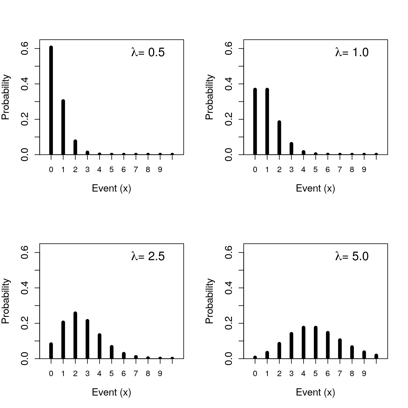
Figure 15.7: Poisson probability distributions given different rate parameter values.
Like the binomial distribution, the Poisson distribution can also be defined mathematically18. Also like the binomial distribution, probabilities in the Poisson distribution focus on discrete observations. This is, probabilities are assigned to a specific number of successes in a set of trials (binomial distribution) or the number of events over time (Poisson distribution). In both cases, the probability distribution focuses on countable numbers. In other words, it does not make any sense to talk about the probability of a coin landing on heads 3.75 times after 10 flips, nor the probability of 2.21 runners passing by a park bench in a given minute. The probability of either of these events happening is zero, which is why Figures 15.5–15.7 all have spaces between the vertical bars. These spaces indicate that values between the integers are impossible. When observations are discrete like this, they are defined by a probability mass function. In the next section, we consider distributions with a continuous range of possible sample values; these distributions are defined by a probability density function.
15.4.3 Uniform distribution
We now move on to continuous distributions, starting with the continuous uniform distribution. I introduce this distribution mainly to clarify the difference between a discrete and continuous distribution. While the uniform distribution is very important for a lot of statistical tools (notably, simulating pseudorandom numbers), it is not something that we come across much in biological or environmental science data. The continuous uniform distribution has two parameters, \(\alpha\) and \(\beta\) (Miller & Miller, 2004).19 Values of \(\alpha\) and \(\beta\) can be any real number (not just integers). For example, suppose that \(\alpha = 1\) and \(\beta = 2.5\). In this case, Figure 15.8 shows the probability distribution for sampling some value \(x\).
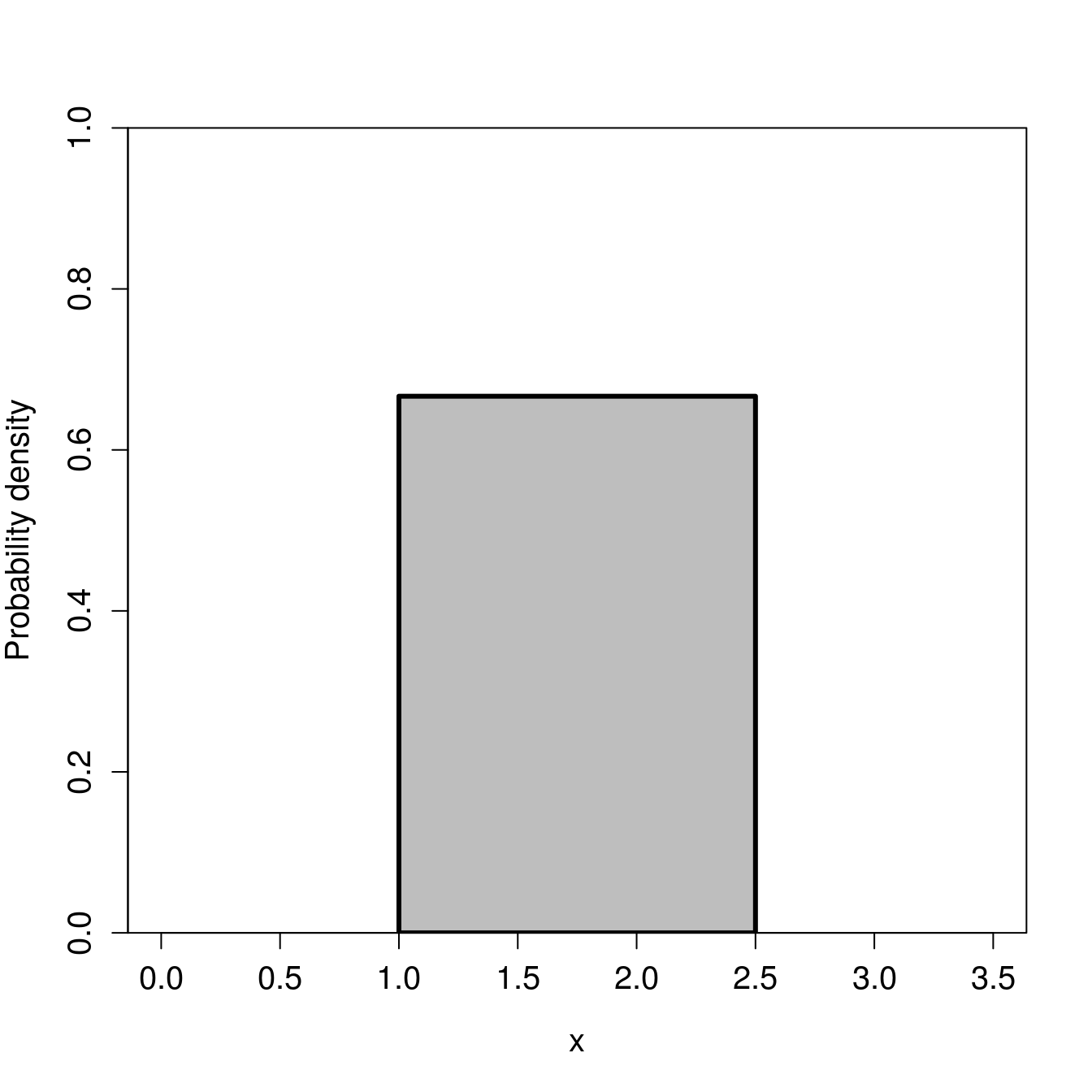
Figure 15.8: A continuous uniform distribution in which a random variable X takes a value between 1 and 2.5.
The height of the distribution in Figure 15.8 is \(1/(\beta - \alpha) = 1/(2.5 - 1) \approx 0.667\). All values between 1 and 2.5 have equal probability of being sampled.
Here is a good place to point out the difference between the continuous distribution versus the discrete binomial and Poisson distributions. From the uniform distribution of Figure 15.8, we can, theoretically, sample any real value between 1 and 2.5 (e.g., 1.34532 or 2.21194; the sampled value can have as many decimals as our measuring device allows). There are uncountably infinite real numbers, so it no longer makes sense to ask what is the probability of sampling a specific number. For example, what is the probability of sampling a value of exactly 2, rather than, say, 1.999999 or 2.000001, or something else arbitrarily close to 2? The probability of sampling a specific number exactly is negligible. Instead, we need to think about the probability of sampling within intervals. For example, what is the probability of sampling a value between 1.9 and 2.1, or any value greater than 2.2? This is the nature of probability when we consider continuous distributions.
15.4.4 Normal distribution
The last distribution, the normal distribution (also known as the ‘Gaussian distribution’ or the ‘bell curve’) has a unique role in statistics (Miller & Miller, 2004; Navarro & Foxcroft, 2022). It appears in many places in the biological and environmental sciences and, partly due to the central limit theorem (see Chapter 16), is fundamental to many statistical tools. The normal distribution is continuous, just like the continuous uniform distribution from the previous section. Unlike the uniform distribution, with the normal distribution, it is possible (at least in theory) to sample any real value, \(-\infty < x < \infty\). The distribution has a symmetrical, smooth bell shape (Figure 15.8), in which probability density peaks at the mean, which is also the median and mode of the distribution. The normal distribution has two parameters: the mean (\(\mu\)) and the standard deviation (\(\sigma\)).20 The mean determines where the peak of the distribution is, and the standard deviation determines the width or narrowness of the distribution. Note that we are using \(\mu\) for the mean here instead of \(\bar{x}\), and \(\sigma\) for the standard deviation instead of \(s\), to differentiate the population parameters from the sample estimates of Chapter 11 and Chapter 12.
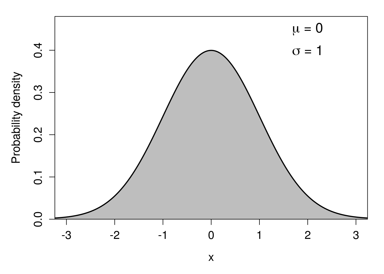
Figure 15.9: A standard normal probability distribution, which is defined by a mean value of 0 and a standard deviation of 1.
The normal distribution shown in Figure 15.9 is called the standard normal distribution, which means that it has a mean of 0 (\(\mu = 0\)) and a standard deviation of 1 (\(\sigma = 1\)). Note that because the standard deviation of a distribution is the square-root of the variance (see Chapter 12), and \(\sqrt{1} = 1\), the variance of the standard normal distribution is also 1. We will look at the standard normal distribution more closely in Chapter 16.
15.5 Summary
This chapter has introduced probability models and different types of distributions. It has focused on the key points that are especially important for understanding and implementing statistical techniques. As such, a lot of details have been left out. For example, the probability distributions considered in Section 15.4 comprise only a small number of example distributions that are relevant for biological and environmental sciences. In Chapter 16, we will get an even closer look at the normal distribution and why it is especially important.
References
In the interest of transparency, this book presents a frequentist interpretation of probability (Mayo, 1996). While this approach does reflect the philosophical inclinations of the author, the reason for working from this interpretation has more to do with the statistical tests that are most appropriate for an introductory statistics book, which are also the tests most widely used in the biological and environmental sciences.↩︎
For those interested, more technically, we can say that a random variable \(X\) has a binomial distribution if and only if its probability mass function is defined by (Miller & Miller, 2004), \[b \left(x; n, \theta \right) = {n \choose x} \theta^{x} \left(1 - \theta\right)^{n-x}.\] In this binomial probability mass function, \(x = 0, 1, 2, ..., n\) (i.e., \(x\) can take any integer value from 0 to n). Note that the \(n\) over the \(x\) in the first parentheses on the right-hand side of the equation is a binomial coefficient, which can be read ‘n choose x’. This can be written out as, \[{n \choose x} = \frac{n!}{x!(n - x)!}.\] The exclamation mark indicates a factorial, such that \(n! = n \times (n-1) \times (n - 2) \times ... \times 2 \times 1\). That is, the factorial multiplies every decreasing integer down to 1. For example, \(4! = 4 \times 3 \times 2 \times 1 = 24\). None of this is critical to know for applying statistical techniques to biological and environmental science data, but it demonstrates just a bit of the theory underlying statistical tools.↩︎
A random variable \(X\) has a Poisson distribution if and only if its probability mass function is defined by (Miller & Miller, 2004), \[p \left(x; \lambda \right) = \frac{\lambda^{x}e^{x}}{x!}.\] Recall from Chapter 1 Euler’s number, \(e \approx 2.718282\), and from the previous footnote that the exclamation mark indicates a factorial. In the Poisson probability mass function, \(x\) can take any integer value greater than or equal to 0.↩︎
A random variable \(X\) has a continuous uniform distribution if and only if its probability density function is defined by (Miller & Miller, 2004), \[u\left(x; \alpha, \beta\right) = \frac{1}{\beta - \alpha},\] where \(\alpha < x < \beta\), and \(u\left(x; \alpha, \beta\right) = 0\) everywhere else. The value \(x\) can take any real number.↩︎
A random variable \(X\) has a normal distribution if and only if its probability density function is defined by (Miller & Miller, 2004), \[n\left(x; \mu, \sigma\right) = \frac{1}{\sigma\sqrt{2\pi}}e^{-\frac{1}{2}\left(\frac{x - \mu}{\sigma}\right)^{2}}.\] In the normal distribution, \(-\infty < x < \infty\). Note the appearance of two irrational numbers introduced back in Chapter 1: \(\pi\) and \(e\).↩︎