Chapter 21 What is hypothesis testing?
Statistical hypotheses are different from scientific hypotheses. In science, a hypothesis should make some kind of testable statement about the relationship between two or more different concepts or observations (Bouma, 2000). For example, we might hypothesise that in a particular population of sparrows, juveniles that have higher body mass will also have higher survival rates. In contrast, statistical hypotheses compare a sample outcome to the outcome predicted given a relevant statistical distribution (Sokal & Rohlf, 1995). That is, we start with a hypothesis that our data are sampled from some distribution, then work out whether or not we should reject this hypothesis. This concept is counter-intuitive, but it is absolutely fundamental for understanding the logic underlying most modern statistical techniques (Greenland et al., 2016; Mayo, 1996; Sokal & Rohlf, 1995), including all subsequent chapters of this book, so we will focus on it here in-depth. The most instructive way to explain the general idea is with the example of coin flips (Mayo, 1996), as we looked at in Chapter 15.
21.1 How ridiculous is our hypothesis?
Imagine that a coin is flipped 100 times. We are told that the coin is fair, meaning that there is an equal probability of it landing on heads or tails (i.e., the probability is 0.5 for both heads and tails in any given flip). From Section 15.4.1, recall that the number of times out of 100 that the coin flip comes up heads will be described by a binomial distribution. The most probable outcome will be 50 heads and 50 tails, but frequencies that deviate from this perfect 50:50 ratio (e.g., 48 heads and 52 tails) are also expected to be fairly common (Figure 21.1).
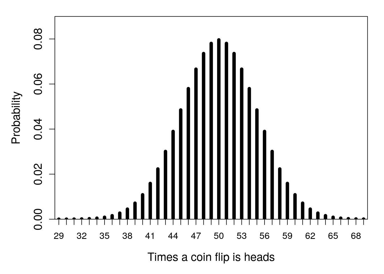
Figure 21.1: Probability distribution for the number of times that a flipped coin lands on heads in 100 trials. Note that some areas of parameter space on the x-axis are cut off because the probabilities associated with this number of flips out of 100 being heads are so low.
The distribution in Figure 21.1 is what we expect to happen if the coin we are flipping 100 times is actually fair. In other words, it is the predicted distribution of outcomes if our hypothesis that the coin is fair is true (more on that later). Now, suppose that we actually run the experiment; we flip the coin in question 100 times. Perhaps we observe heads 30 times out of the 100 total flips. From the distribution in Figure 21.1, this result seems very unlikely if the coin is actually fair. If we do the maths, the probability of observing 30 heads or fewer (i.e., getting anywhere between 0 and 30 heads total) is only \(P = 0.0000392507\). And the probability of getting this much of a deviation from 50 heads (i.e., either 20 less than or 20 more than 50) is \(P = 0.0000785014\) (two times 0.0000392507, since the binomial distribution is symmetrical around 50). This seems a bit ridiculous! Do we really believe that the coin is fair if the probability of getting a result this extreme is so low?
Getting 30 head flips is maybe a bit extreme. What if we flip the coin 100 times and get 45 heads? In this case, if the coin is fair, then we would predict this number of heads or fewer with a probability of about \(P = 0.0967\) (i.e., about 9.67% of the time, we would expect to get 45 or fewer heads). And we would predict a deviation as extreme as 5 from the 50:50 ratio of heads to tails with a probability of about \(P = 0.193\) (i.e., about 19.3% of the time, we would get 45 heads or fewer, or 55 heads or more). This does not sound nearly so unrealistic. If a fair coin will give us this much of a deviation from the expected 50 heads and 50 tails about 20% of the time, then perhaps our hypothesis is not so ridiculous, and we can conclude the coin is indeed fair.
How improbable does our result need to be to cause us to reject our hypothesis that the coin is fair? There is no definitive answer to this question. In the biological and environmental sciences, we traditionally use a probability of 0.05, but this threshold is completely arbitrary40. All it means is that we are willing to reject our hypothesis (i.e., declare the coin to be unfair) when it is actually true (i.e., the coin really is fair) about 5% of the time. Note that we do need to decide on some finite threshold for rejecting our hypothesis because even extremely rare events, by definition, can sometimes happen. In the case of 100 coin flips, there is always a small probability of getting any number of heads from a fair coin (although getting zero heads would be extraordinarily rare, \(P \approx 7.89 \times 10^{-31}\), i.e., a decimal followed by 30 zeros, then a 7). We can therefore never be certain about rejecting or not rejecting the hypothesis that we have a fair coin.
This was a very concrete example intended to provide an intuitive way of thinking about hypothesis testing in statistics. In the next section, we will look more generally at what hypothesis testing means in statistics and the terminology associated with it. But everything that follows basically relies on the same general logic as the coin-flipping example here; if our hypothesis is true, then what is the probability of our result?
21.2 Statistical hypothesis testing
A statistical test is used to decide if we should reject the hypothesis that some observed value or calculated statistic was sampled from a particular distribution (Sokal & Rohlf, 1995). In the case of the coin example in the previous section, the observed value was the number of heads, and the distribution was the binomial distribution. In other cases, we might, e.g., test the hypothesis that a value was sampled from a normal or t-distribution. In all of these cases, the hypothesis that we are testing is the null hypothesis, which we abbreviate as \(H_{0}\) (e.g., the coin is fair). Typically, \(H_{0}\) is associated with the lack of an interesting statistical pattern, such as when a coin is fair, when there is no difference between two groups of observations, or when two variables are not associated with each other. This null hypothesis contrasts an alternative hypothesis, which we abbreviate as \(H_{A}\) (e.g., the coin is not fair). Alternative hypotheses are always defined by some relationship to \(H_{0}\) (Sokal & Rohlf, 1995). Typically, \(H_{A}\) is associated with something interesting happening, such as a biased coin, a difference between groups of observations, or an association between two variables. Table 21.1 below presents some null and alternative hypotheses that might be relevant in the biological or environmental sciences.
| Null Hypothesis \(H_{0}\) | Alternative Hypothesis \(H_{A}\) |
|---|---|
| There is no difference between juvenile and adult sparrow mortality | Mortality differs between juvenile and adult sparrows |
| Amphibian body size does not change with increasing latitude | Amphibian body size increases with latitude |
| Soil nitrogen concentration does not differ between agricultural and non-agricultural fields | Soil nitrogen concentration is lower in non-agricultural fields |
Notice that alternative hypotheses can indicate direction (e.g., amphibian body size will increase with latitude, or nitrogen content will be lower in non-agricultural fields), or they can be non-directional (e.g., mortality will be different based on life-history stage). When our alternative hypothesis indicates direction, we say that the hypothesis is one-sided. This is because we are looking at one side of the null distribution. In the case of our coin example, a one-sided \(H_{A}\) might be that the probability of flipping heads is less than 0.5, meaning that we reject \(H_{0}\) only given numbers on the left side of the distribution in Figure 21.1 (where the number of times a coin flip is heads is fewer than 50). A different one-sided \(H_{A}\) would be that the probability of flipping heads is greater than 0.5, in which case we would reject \(H_{0}\) only given numbers on the right side of the distribution. In contrast, when our alternative hypothesis does not indicate direction, we say that the hypothesis is two-sided. This is because we are looking at both sides of the null distribution. In the case of our coin example, we might not care in which direction the coin is biased (towards heads or tails), just that the probability of flipping heads does not equal 0.5. In this case, we reject \(H_{0}\) at both extremes of the distribution of Figure 21.1.
21.3 P-values, false positives, and power
In our hypothetical coin-flipping example, we used \(P\) to indicate the probability of getting a particular number of heads out of 100 total flips if our coin was fair. This \(P\) (sometimes denoted with a lower-case \(p\)) is what we call a ‘p-value’.
A p-value is the probability of getting a result as or more extreme than the one observed assuming \(H_{0}\) is true.41
This is separated and in bold because it is a very important concept in statistics, and it is one that is very, very easy to misinterpret42. A p-value is not the probability that the null hypothesis is true (we actually have no way of knowing this probability). It is also not the probability that an alternative hypothesis is false (we have no way of knowing this probability either). A p-value specifically assumes that the null hypothesis is true, then asks what the probability of an observed result would be conditional upon this assumption. In the case of our coin flipping example, we cannot really know the probability that the coin is fair or unfair (depending on your philosophy of statistics, this might not even make conceptual sense). But we can say that if the coin is fair, then an observation of \(\leq 45\) would occur with a probability of \(P = 0.0967\).
Before actually calculating a p-value, we typically set a threshold level (\(\alpha\)) below which we will conclude that our p-value is statistically significant43. As mentioned in Section 21.1, we traditionally set \(\alpha= 0.05\) in the biological and environmental sciences (although rarely \(\alpha = 0.01\) is used). This means that if \(P < 0.05\), then we reject \(H_{0}\) and conclude that our observation is statistically significant. It also means that even when \(H_{0}\) really is true (e.g., the coin really is fair), we will mistakenly reject \(H_{0}\) with a probability of 0.05 (i.e., 5% of the time). This is called a Type I error (i.e., false positive), and it typically means that we will infer a pattern of some kind (e.g., difference between groups, or relationship between variables) where none really exists. This is obviously an error that we want to avoid, which is why we set \(\alpha\) to a low value.
In contrast, we can also fail to reject \(H_{0}\) when \(H_{A}\) is actually true. That is, we might mistakenly conclude that there is no evidence to reject the null hypothesis when the null hypothesis really is false. This is called a Type II error. The probability that we commit a Type II error, i.e., that we fail to reject the null hypothesis when it is false, is given the symbol \(\beta\). Since \(\beta\) is the probability that we fail to reject \(H_{0}\) when it is false, \(1 - \beta\) is the probability that we do reject \(H_{0}\) when it is false. This \(1 - \beta\) is the statistical power of a test. Note that \(\alpha\) and \(\beta\) are not necessarily related to each other. Our \(\alpha\) is whatever we set it to be (e.g., \(\alpha = 0.05\)). But statistical power will depend on the size of the effect that we are measuring (e.g., how much bias there is in a coin if we are testing whether or not it is fair), and on the size of our sample. Increasing our sample size will always increase our statistical power, i.e., our ability to reject the null hypothesis when it is really false. Table 21.2 illustrates the relationship between whether or not \(H_{0}\) is true, and whether or not we reject it.
| Do Not Reject \(H_{0}\) | Reject \(H_{0}\) | |
|---|---|---|
| \(H_{0}\) is true | Correct decision | Type I error |
| \(H_{0}\) is false | Type II error | Correct decision |
Note that we never accept a null hypothesis; we just fail to reject it. Statistical tests are not really set up in a way that \(H_{0}\) can be accepted44. The reason for this is subtle, but we can see the logic if we again consider the case of the fair coin. If \(H_{0}\) is true, then the probability of flipping heads is \(P(heads) = 0.5\) (i.e., \(H_{0}:\:P(heads) = 0.5\)). But even if we fail to reject \(H_{0}\), this does not mean that we can conclude with any real confidence that our null hypothesis \(P(heads) = 0.5\) is true. What if we instead tested the null hypothesis that our coin was very slightly biased, such that \(H_{0}:\:P(heads) = 0.4999\)? If we failed to reject the null hypothesis that \(P(heads) = 0.5\), then we would probably also fail to reject a \(H_{0}\) that \(P(heads) = 0.4999\). There is no way to meaningfully distinguish between these two potential null hypotheses by just testing one of them. We therefore cannot conclude that \(H_{0}\) is correct; we can only find evidence to reject it. In contrast, we can reasonably accept an alternative hypothesis \(H_{A}\) when we reject \(H_{0}\).
References
I have heard many apocryphal stories about how a probability of 0.05 was decided upon, but I have no idea which, if any, of these stories are actually true.↩︎
Technically, it also assumes that all of the assumptions of the model underlying the hypothesis test are true, but we will worry about this later.↩︎
In fact, the p-value is so easy to misinterpret and so widely misused, that some scientists have called for them to be abandoned entirely (Wasserstein & Lazar, 2016), but see Stanton-Geddes et al. (2014) and Mayo (2019).↩︎
Like p-values, setting thresholds below which we consider \(P\) to be significant is at least somewhat controversial (Mayo, 2021; McShane et al., 2019). But the use of statistical significance thresholds is ubiquitous in the biological and environmental sciences, so we will use them throughout this book (it is important to understand them and interpret them).↩︎
Note that we might, for non-statistical reasons, conclude the absence of a particular phenomenon or relationship between observations. For example, following a statistical test, we might become convinced that a coin really is fair, or that there is no relationship between sparrow body mass and survival. But these are conclusions about scientific hypotheses, not statistical hypotheses.↩︎