Chapter 33 Multiple regression
Multiple regression is an extension of the general idea of simple linear regression, with some important caveats. In multiple regression, there is more than one independent variable (\(x\)), and each independent variable is associated with its own regression coefficient (\(b\)). For example, if we have two independent variables, \(x_{1}\) and \(x_{2}\), then we can predict \(y\) using the equation,
\[y = b_{0} + b_{1}x_{1} + b_{2}x_{2}.\]
More generally, for \(k\) independent variables,
\[y = b_{0} + b_{1}x_{1} + ... + b_{k}x_{k}.\]
Mathematically, this almost seems like a trivial extension of the simple linear regression model. But conceptually, there is an additional consideration necessary to correctly interpret the regression coefficients (i.e., \(b\) values). Values of \(b_{i}\) now give us the predicted effects of \(x_{i}\) if all other independent variables were to be held constant (Sokal & Rohlf, 1995). In other words, \(b_{i}\) tells us what would happen if we were to increase \(x_{i}\) by a value of 1 in the context of every other independent variable in the regression model. We call these \(b\) coefficients partial regression coefficients. The word ‘partial’ is a general mathematical term meaning that we are only looking at the effect of a single independent variable (Borowski & Borwein, 2005). Since multiple regression investigates the effect of each independent variable in the context of all other independent variables, we might sometimes expect regression coefficients to be different from what they would be given a simple linear regression (Morrissey & Ruxton, 2018). It is even possible for the sign of the coefficients to change (e.g., from negative to positive).
To illustrate a multiple regression, consider again the fig fruit volume example from Chapter 32 (Duthie & Nason, 2016). Suppose that in addition to latitude, altitude was also measured in metres for each fruit (Table 33.1).
| Latitude | 23.7 | 24.0 | 27.6 | 27.2 | 29.3 | 28.2 | 28.3 |
| Altitude | 218.5 | 163.5 | 330.1 | 542.3 | 656.0 | 901.3 | 709.6 |
| Volume | 2399.0 | 2941.7 | 2167.2 | 2051.3 | 1686.2 | 937.3 | 1328.2 |
We can use a scatterplot to visualise each independent variable on the x-axis against the dependent variable on the y-axis (Figure 33.1).
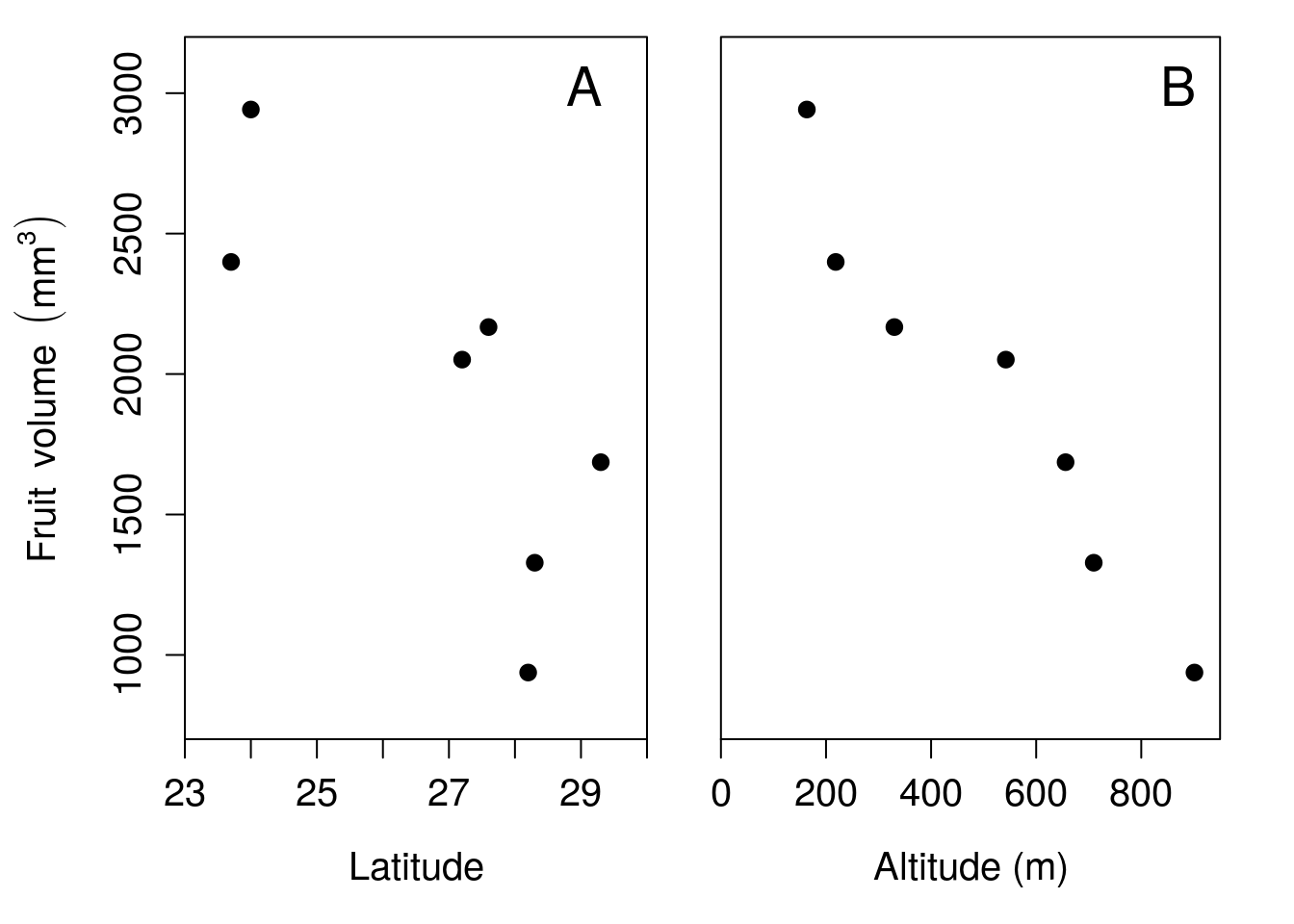
Figure 33.1: Relationship between latitude and fruit volume for seven fig fruits collected from Baja, Mexico in 2010, and the relationship between altitude and fruit volume for the same dataset.
As with simple regression (Chapter 32), we can test whether or not the overall model that includes both latitude and altitude as independent variables produces a significantly better fit to the data than just the mean volume. We can also find partial regression coefficients for latitude (\(b_{1}\)) and altitude (\(b_{2}\)), and test whether or not these coefficients are significantly different from 0.
In Chapter 32, we found that a simple regression of latitude against fruit volume had an intercept of \(b_{0} = 8458.3\) and a regression coefficient of \(b_{1} = -242.68\),
\[Volume = 8458.3 - 242.68(Latitude).\]
The slope of the regression line (\(b_{1}\)) was significantly different from zero (\(P = 0.03562\)).
A multiple regression can be used with latitude and altitude as independent variables to predict volume,
\[Volume = b_{0} + b_{1}(Latitude) + b_{2}(Altitude).\]
We have the values of volume, latitude, and altitude in Table 33.1. We now need to run a multiple regression to find the intercept (\(b_{0}\)) and partial regression coefficients describing the partial effects of latitude (\(b_{1}\)) and altitude (\(b_{2}\)) on volume. In jamovi, running a multiple regression is just a matter of including the additional independent variable (Altitude, in this case). Table 33.2 shows an output table, which gives us estimates of \(b_{0}\), \(b_{1}\), and \(b_{2}\) (column ‘Estimate’), along with p-values for the intercept and each partial regression coefficient (column ‘Pr(>|t|)’).
| Estimate | Std. Error | t Value | Pr(>|t|) | |
|---|---|---|---|---|
| (Intercept) | 2988 | 1698 | 1.76 | 0.1532 |
| Latitude | 5.588 | 71.49 | 0.07816 | 0.9415 |
| Altitude | -2.402 | 0.5688 | -4.223 | 0.01344 |
There are a few things to point out from Table 33.2. First, note that as with simple linear regression (see Section 32.7), the significance of the intercept and regression coefficients is tested using the t-distribution. This is because we assume that these sample coefficients (\(b_{0}\), \(b_{1}\), and \(b_{2}\)) will be normally distributed around the true population parameter values (\(\beta_{0}\), \(\beta_{1}\), and \(\beta_{2}\)). In other words, if we were to go back out and repeatedly collect many new datasets (sampling volume, latitude, and altitude ad infinitum), then the distribution of \(b\) sample coefficients calculated from these datasets would be normally distributed around the true \(\beta\) population coefficients. The t-distribution, which accounts for uncertainty that is attributable to a finite sample size (see Chapter 19), is therefore the correct one to use when testing the significance of coefficients.
Second, the intercept has changed from what it was in the simple linear regression model. In the simple linear regression, it was 8458.30961, but in the multiple regression it is \(b_{0} = 2988.24539\). The p-value of the intercept has also changed. In the simple linear model, the p-value was significant (\(P = 0.0142\)). But in the multiple regression model, it is not significant (\(P = 0.1532\)).
Third, and perhaps most strikingly, the prediction and significance of latitude has changed completely. In the simple linear regression model from Section 32.7.4, fruit volume decreased with latitude (\(b_{1} = -242.68\)), and this decrease was statistically significant (\(P = 0.0356\)). Now the multiple regression output is telling us that, if anything, fruit volume appears to increase with latitude (\(b_{1} = 5.59\)), although this is not statistically significant (\(P = 0.9415\)). What is going on here? This result illustrates the context dependence of partial regression coefficients in the multiple regression model. In other words, although fruit volume appeared to significantly decrease with increasing latitude in the simple regression model of Chapter 32, this is no longer the case once we account for the altitude from which the fruit was collected. Latitude, by itself, does not appear to affect fruit volume after all. It only appeared to affect fruit volume because locations at high latitude also tend to be higher in altitude. And each metre of altitude appears to decrease fruit volume by about 2.4 \(\mathrm{mm}^{3}\) (Table 33.2). This partial effect of altitude on fruit volume is statistically significant (\(P < 0.05\)). We therefore do not reject the null hypothesis that the intercept (\(b_{0}\)) and partial coefficient of latitude (\(b_{1}\)) is significantly different from 0. But we do reject the null hypothesis that \(b_{2} = 0\), and we can conclude that altitude has an effect on fig fruit volume.
We can also look at the overall multiple regression model. Figure 33.2 shows what this model output looks like reported by jamovi (The jamovi project, 2024).
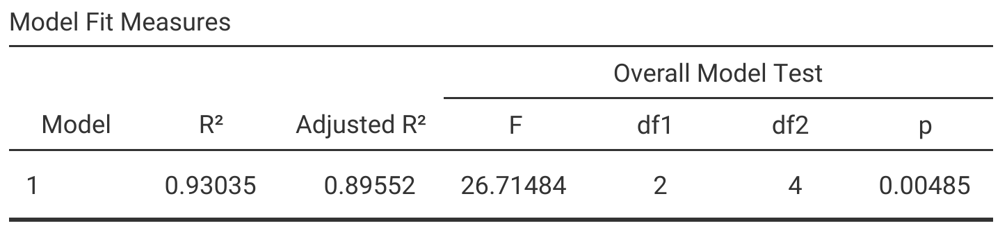
Figure 33.2: Jamovi output table for a multiple linear regression in which latitude and altitude are independent variables and fig fruit volume is a dependent variable.
As with the simple linear regression output from Chapter 32.7.4, the overall model test output table includes columns for \(R^{2}\), \(F\), degrees of freedom, and a p-value for the overall model. There is one key difference between this output table and the overall model output for a simple linear regression, and that is the Adjusted \(R^{2}\). This is the adjusted coefficient of determination \(R^{2}_{\mathrm{adj}}\), which is necessary to compare regression models with different numbers of independent variables.
33.1 Adjusted coefficient of determination
Recall from Section 32.5 that the coefficient of determination (\(R^{2}\)) tells us how much of the total variation in the dependent variable is explained by the regression model. This was fine for a simple linear regression, but with the addition of new independent variables, the proportion of the variance in y explained by our model is expected to increase even if the new independent variables are not very good predictors. This is because the amount of variation explained by our model can only increase if we add new independent variables. In other words, any new independent variable that we choose to add to the model cannot explain a negative amount of variation; that does not make any sense! The absolute worst that an independent variable can do is explain zero variation. And even if the independent variable is just a set of random numbers, it will likely explain some of the variation in the dependent variable just by chance. Hence, even if newly added independent variables are bad predictors, they might still improve the goodness of fit of our model by chance. To help account for this spurious improvement of fit, we can use an adjusted R squared (\(R^{2}_{\mathrm{adj}}\)). The \(R^{2}_{\mathrm{adj}}\) takes into account the \(R^{2}\), the sample size (\(N\)), and the number of independent variables (\(k\)),
\[R^{2}_{\mathrm{adj}} = 1 - \left(1 - R^{2}\right)\left(\frac{N - 1}{N - k - 1}\right).\]
As \(k\) increases, the value of \((N-1)/(N-k-1)\) gets bigger. And as this fraction gets bigger, we are subtracting a bigger value from 1, so \(R^{2}_{\mathrm{adj}}\) decreases. Consequently, more independent variables cause a decrease in the adjusted R-squared value. This attempts to account for the inevitable tendency of \(R^{2}\) to increase with \(k\).