Chapter 3 Practical. Preparing data
In this chapter, we will use a spreadsheet to organise datasets following the tidy approach explained in Chapter 2, then save these datasets as CSV files to be opened in jamovi statistical software (The jamovi project, 2024). The data organisation in this chapter can be completed using LibreOffice Calc, MS Excel, or Google Sheets. The screenshots below will be from LibreOffice Calc, but the instructions provided will work on any of the three aforementioned spreadsheet programs.
There are four data exercises in this chapter. All of these exercises will focus on organising data into a tidy format. Exercise 3.1 uses handwritten field data that need to be entered into a spreadsheet in a tidy format. These data include information shown in Figure 2.2, plus tallies of seed counts. The goal is to get all of this information into a tidy format and save it as a CSV file. Exercise 3.2 presents some data on the number of eggs produced by five different fig wasp species (more on these in Chapter 8). The data are in an untidy format, so the goal is to reorganise them and save them as a tidy CSV file. Exercise 3.3 presents counts of the same five fig wasp species as in Exercise 3.2, which need to be reorganised in a tidy format. Exercise 3.4 presents data that are even more messy. These are morphological measurements of the same five species of wasps, including lengths and widths of wasp heads, thoraxes, and abdomens. The goal in this exercise is to tidy the data, then estimate total wasp volume from the morphological measurements using mathematical formulas, keeping in mind the order of operations from Chapter 1.
3.1 Transferring data to a spreadsheet
Exercise 3.1 focuses on data collected from the fruits of fig trees collected from Baja, Mexico in 2010 (Duthie et al., 2015; Duthie & Nason, 2016). Due to the nature of the work, the data needed to be recorded in notebooks and collected in two different locations. The first location was the field, where data were collected identifying tree locations and fruit dimensions. Baja is hot and sunny (Figure 3.1).
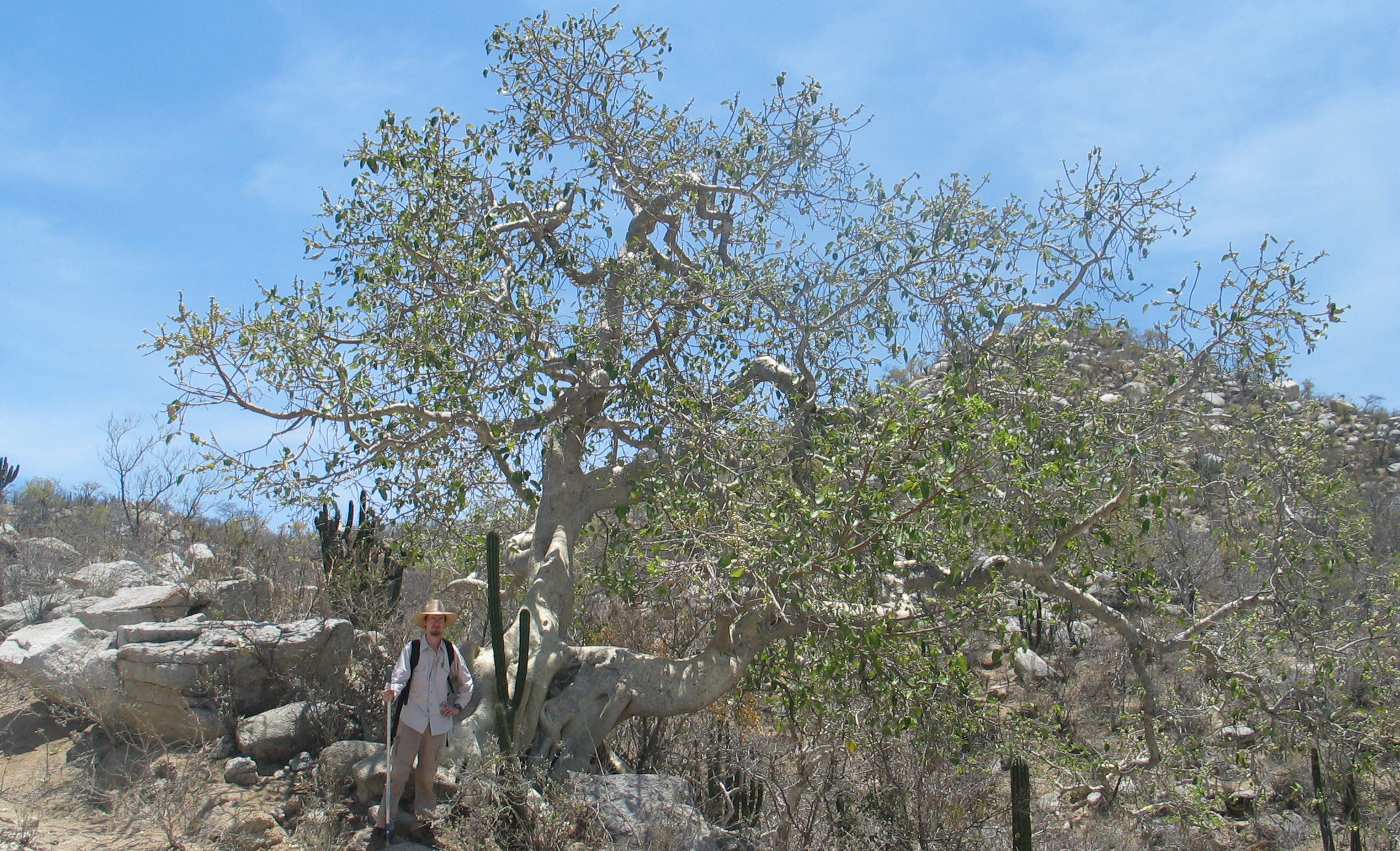
Figure 3.1: Fully grown Sonoran Desert Rock Fig in the desert of Baja, Mexico.
Fruit measurements were made with a ruler and recorded in a field notebook. These measurements are shown in Figure 3.2.
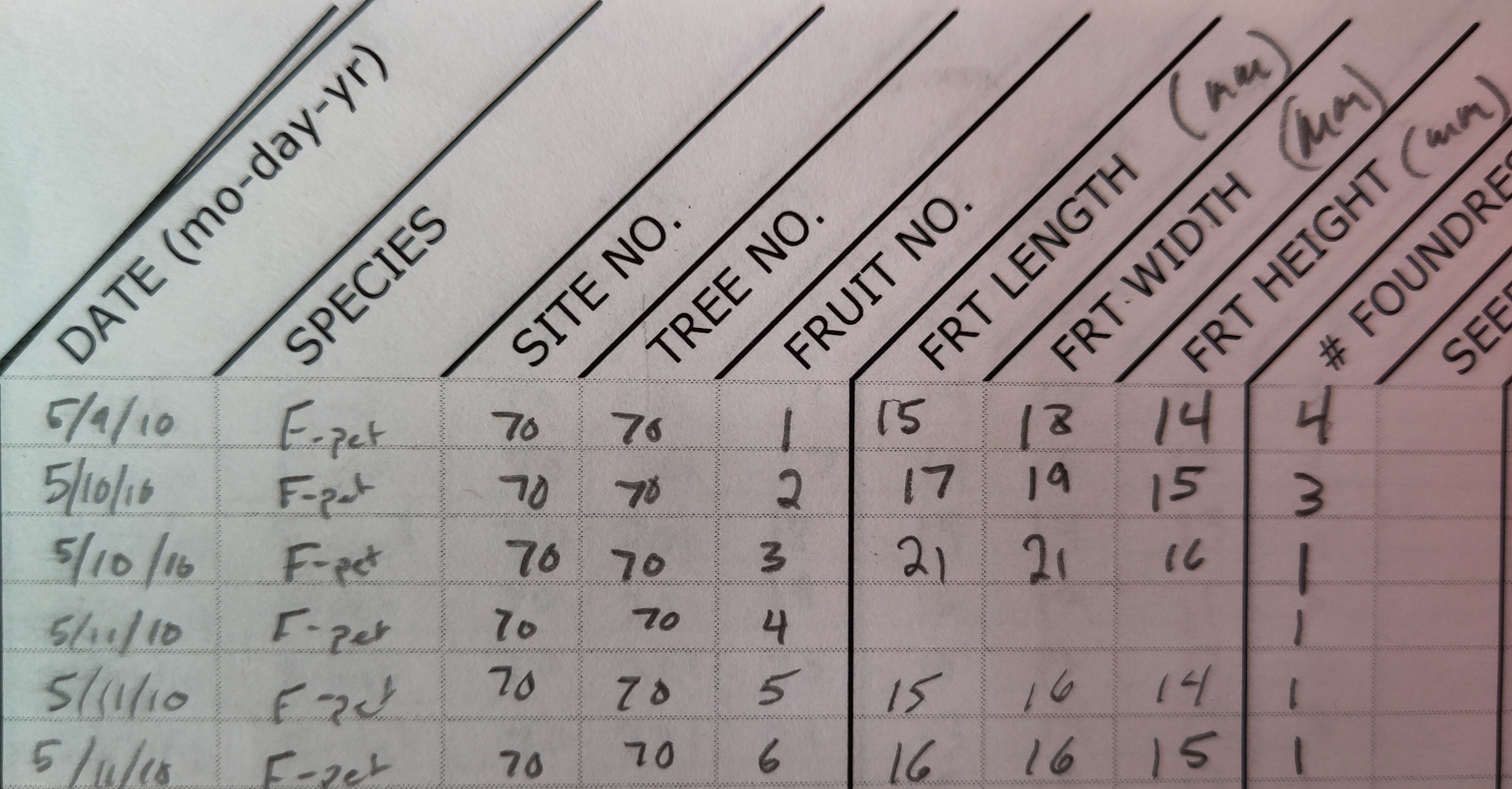
Figure 3.2: Portion of a lab notebook used to record measurements of fig fruits from different trees in 2010.
The second location was in a lab in Iowa, USA. Fruits were dried and shipped to Iowa State University so that seeds could be counted under a microscope. Counts were originally recorded as tallies in a lab notebook. The goal of Exercise 3.1 is to get all of this information into a single tidy spreadsheet.
The best place to start is with an empty spreadsheet, so open a new one in LibreOffice Calc, MS Excel, or Google Sheets. Remember that each row will be a unique observation; in this case, a unique fig fruit from which measurements were recorded. Each column will be a variable of that observation. Fortunately, the data in Figure 3.2 are already looking quite tidy. The information here can be put into the spreadsheet mostly as written in the notebook. But there are a few points to keep in mind:
- It is important to start in column A and row 1; do not leave any empty rows or columns because when we get to the statistical analysis in jamovi, jamovi will assume that these empty rows and columns signify missing data.
- There is no need to include any formatting (e.g., bold, underline, colour) because it will not be saved in the CSV or recognised by jamovi.
- Missing information, such as the empty boxes for the fruit dimensions in row 4 in the notebook (Figure 3.2), should be indicated with an ‘
NA’ (capital letters, but without the quotes). This will let jamovi know that these data are missing. - The date is written in an American style of month-day-year, which might get confusing. It might be better to have separate columns for year, month, and day, and to write out the full year (2010).
The column names in Figure 3.2 are (1) Date, (2) Species, (3) Site number, (4) Tree number, (5) Fruit length in millimetres, (6) Fruit width in millimetres, and (7) Fruit height in millimetres. All of the species are Ficus petiolaris, which is abbreviated to ‘F-pet’ in the field notebook. How you choose to write some of this information down is up to you (e.g., date format, capitalisation of column names), but when finished, the spreadsheet should be organised like the one in Figure 3.3.
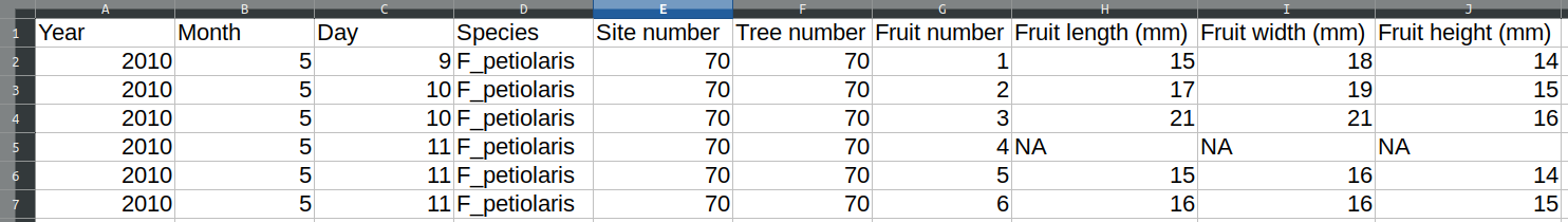
Figure 3.3: Spreadsheet with data organised in a tidy format and nearly ready for analysis.
This leaves us with the data that had to be collected later in the lab. Small seeds needed to be meticulously separated from other material in the fig fruit, then tallied under a microscope. Tallies from this notebook are recreated below.
Site 70, Tree 70, Fruit 1: 238 total
ᚎ ᚎ ᚎ ᚎ ᚎ ᚎ ᚎ ᚎ ᚎ ᚎ ᚎ ᚎ ᚎ ᚎ ᚎ ᚎ ᚎ ᚎ ᚎ ᚎ
 ᚎ ᚎ ᚎ ᚎ ᚎ ᚎ ᚎ ᚎ ᚎ ᚎ ᚎ ᚎ ᚎ ᚎ ᚎ ᚎ ᚎ ᚎ ᚎ ᚎ
 ᚎ ᚎ ᚎ ᚎ ᚎ ᚎ ᚎ 𝍫
Site 70, Tree 70, Fruit 2: 198 total
ᚎ ᚎ ᚎ ᚎ ᚎ ᚎ ᚎ ᚎ ᚎ ᚎ ᚎ ᚎ ᚎ ᚎ ᚎ ᚎ ᚎ ᚎ ᚎ ᚎ
 ᚎ ᚎ ᚎ ᚎ ᚎ ᚎ ᚎ ᚎ ᚎ ᚎ ᚎ ᚎ ᚎ ᚎ ᚎ ᚎ ᚎ ᚎ ᚎ 𝍫
Site 70, Tree 70, Fruit 3: 220 total
ᚎ ᚎ ᚎ ᚎ ᚎ ᚎ ᚎ ᚎ ᚎ ᚎ ᚎ ᚎ ᚎ ᚎ ᚎ ᚎ ᚎ ᚎ ᚎ ᚎ
 ᚎ ᚎ ᚎ ᚎ ᚎ ᚎ ᚎ ᚎ ᚎ ᚎ ᚎ ᚎ ᚎ ᚎ ᚎ ᚎ ᚎ ᚎ ᚎ ᚎ
 ᚎ ᚎ ᚎ ᚎ
Site 70, Tree 70, Fruit 4: 169 total
ᚎ ᚎ ᚎ ᚎ ᚎ ᚎ ᚎ ᚎ ᚎ ᚎ ᚎ ᚎ ᚎ ᚎ ᚎ ᚎ ᚎ ᚎ ᚎ ᚎ
 ᚎ ᚎ ᚎ ᚎ ᚎ ᚎ ᚎ ᚎ ᚎ ᚎ ᚎ ᚎ ᚎ 𝍬
Site 70, Tree 70, Fruit 5: 188 total
ᚎ ᚎ ᚎ ᚎ ᚎ ᚎ ᚎ ᚎ ᚎ ᚎ ᚎ ᚎ ᚎ ᚎ ᚎ ᚎ ᚎ ᚎ ᚎ ᚎ
 ᚎ ᚎ ᚎ ᚎ ᚎ ᚎ ᚎ ᚎ ᚎ ᚎ ᚎ ᚎ ᚎ ᚎ ᚎ ᚎ ᚎ 𝍫
Site 70, Tree 70, Fruit 6: 139 total
ᚎ ᚎ ᚎ ᚎ ᚎ ᚎ ᚎ ᚎ ᚎ ᚎ ᚎ ᚎ ᚎ ᚎ ᚎ ᚎ ᚎ ᚎ ᚎ ᚎ
 ᚎ ᚎ ᚎ ᚎ ᚎ ᚎ ᚎ 𝍬
Fortunately, the summed tallies have been written next to the site, tree, and fruit, which makes inputting them into a spreadsheet easier. But it is important to also recognise this step as a potential source of human error in data collection. It is possible that the tallies were counted inaccurately, meaning that the tallies do not sum to the numbers reported above. It is always good to be able to go back and check. There are at least two other potential sources of human error in counting seeds and inputting them into the spreadsheet, one before, and one after counting the tallies. Fill in 1 and 3 below with potential causes of error.
- Tallies are not counted correctly in the lab notebook
Next, create a new column in the spreadsheet and call it ‘Seeds’ (use column K). Fill in the seed counts for each of the six rows. The end result will be a tidy dataset that is ready to be saved as a CSV.
What you do next depends on the spreadsheet program that you are using and how you are using it. If you are using LibreOffice Calc or MS Excel on your computer, then you should be able to simply save your file as something like ‘Fig_fruits.csv’, and the program will recognise that you intend to save as a CSV file (in MS Excel, you might need to find the pull-down box for ‘Save as type:’ under the ‘File name:’ box and choose ‘CSV’). If you are using Google Sheets, you can navigate in the toolbar to ‘File \(\to\) Download \(\to\) Comma-separated values (.csv)’, which will start a download of your spreadsheet in CSV format. If you are using MS Excel in a browser online, then it is a bit more tedious. At the time of writing, the online version of MS Excel does not allow users to save or export to a CSV. It will therefore be necessary to save as an XLSX, then convert to CSV later in another spreadsheet program (local version of MS Excel, LibreOffice Calc, or Google Sheets).
Save your file in a location where you know that you can find it again. It might be a good idea to create a new folder on your computer or your cloud storage online for files in this book. This will ensure that you always know where your data files are located and can access them easily.
3.2 Making spreadsheet data tidy
Exercise 3.2 is more self-guided than Exercise 3.1. After reading Chapter 2 and completing Exercise 3.1, you should have a bit more confidence in organising data in a tidy format. Here we will work with a dataset that includes counts of the number of eggs collected from fig wasps, which are small species of insects that lay their eggs into the ovules of fig flowers (Weiblen, 2002). You can download this dataset online1 or recreate it from Table 3.1.
| Het1 | Het2 | LO1 | SO1 | SO2 |
|---|---|---|---|---|
| 35 | 51 | 72 | 50 | 44 |
| 32 | 55 | 76 | 47 | 44 |
| 34 | 52 | 77 | 48 | 46 |
| 38 | 54 | 78 | 54 | 36 |
| 34 | 55 | 76 | 54 | 51 |
| 34 | 54 | 72 | 46 | 50 |
| 34 | 56 | 79 | 50 | 36 |
| 34 | 53 | 76 | 50 | 56 |
| 32 | 54 | 77 | 52 | 58 |
| 30 | 54 | 75 | 51 | 45 |
| 49 | ||||
| 39 | ||||
| 54 | ||||
| 52 |
Using what you have learnt in Chapter 2 and Exercise 3.1, create a tidy version of the wasp egg loads dataset. For a helpful hint, it might be most efficient to open a new spreadsheet and copy and paste information from the old to the new.
How many columns did you need to create the new dataset? _________
Are there any missing data in this dataset? _________
Save the tidy dataset to a CSV file.
3.3 Making data tidy again
Exercise 3.3, like Exercise 3.2, is self-guided. The data are presented in a fairly common, but untidy, format, and the challenge is to reorganise them into a tidy dataset that is ready for statistical analysis. Table 3.2 shows the number of different species of wasps counted in five different fig fruits. Rows list all of the species and columns list the fruits, with the counts in the middle. This is an efficient way to present the data so that they are all easy to see, but this will not work for running statistical analysis.
| Species | Fruit_1 | Fruit_2 | Fruit_3 | Fruit_4 | Fruit_5 |
|---|---|---|---|---|---|
| Het1 | 0 | 0 | 0 | 1 | 0 |
| Het2 | 0 | 2 | 3 | 0 | 0 |
| LO1 | 4 | 37 | 0 | 0 | 3 |
| SO1 | 0 | 1 | 0 | 3 | 2 |
| SO2 | 1 | 12 | 2 | 0 | 0 |
This exercise might be a bit more challenging than Exercise 3.2. The goal is to use the information in Table 3.2 to create a tidy dataset. Remember that each observation (wasp counts, in this case) should get its own row, and each variable should get its own column. Try creating a tidy dataset from the information in Table 3.2, then save the dataset to a CSV file.
3.4 Tidy data and spreadsheet calculations
Exercise 3.4 requires some restructuring and calculations. The dataset that will be used in this exercise includes morphological measurements from five species of fig wasps, the same species used in Exercises 3.2 and 3.3. The dataset for this exercise can be downloaded online2. This dataset is about as untidy as it gets. First note that there are multiple sheets in the spreadsheet, which is not allowed in a CSV file. You can see these sheets by looking at the very bottom of the spreadsheet, which will have separating tabs called Het1, Het2, LO1, SO1, and SO2 (Figure 3.4).

Figure 3.4: Spreadsheets can include multiple sheets. This image shows that the spreadsheet containing information for fig wasp morphology includes five separate sheets, one for each species.
You can click on all of the different tabs to see the measurements of head length, head width, thorax length, thorax width, abdomen length, and abdomen width for wasps of each of the five species. All of the measurements are collected in millimetres. Note that the individual sheets contain text formatting (titles highlighted and in bold), and there is a picture of each wasp in its respective sheet. The formatting and pictures are a nice touch for providing some context, but they cannot be used in statistical analysis. The first task is to create a tidy version of this dataset. Probably the best way to do this is to create a new spreadsheet entirely and copy-paste information from the old. It is a good idea to think about how the tidy dataset will look before getting started. What columns should this new dataset include? Write your answer below.
How many rows are needed? _________________
When you are ready, create the new dataset. Your dataset should have all of the relevant information about wasp head, thorax, and abdomen measurements.
Next comes a slightly more challenging part, which will make use of some of the background mathematics reviewed in Chapter 1. Suppose that we wanted our new dataset to include information about the volumes of each of the three wasp body segments, and wasp total volume. To do this, let us assume that the wasp head is a sphere (it is not, exactly, but this is probably the best estimate that we can get under the circumstances). Calculate the head volume of each wasp using the following formula,
\[V_{\mathrm{head}} = \frac{4}{3}\pi \left(\frac{Head_L + Head_W}{4}\right)^{3}.\]
In the equation above, \(Head_{\mathrm{L}}\) is head length (mm) and \(Head_{\mathrm{W}}\) is head width (note, \((Head_\mathrm{L} + Head_\mathrm{W})/4\) estimates the radius of the head).
You can replace \(\pi\) with the approximation \(\pi \approx 3.14\).
To make this calculation in your spreadsheet, find the cell in which you want to put the head volume.
By typing in the = sign, the spreadsheet will know to start a new calculation or function in that cell.
Try this with an empty cell by typing ‘= 5 + 4’ in it (without quotes).
When you hit ‘Enter’, the spreadsheet will make the calculation for you, and the number in the new cell will be 9.
To see the equation again, you just need to double-click on the cell.
To get an estimate of head volume into the dataset, we can create a new column of data.
To calculate \(V_{\mathrm{head}}\) for the first wasp in row 2 of the spreadsheet, we could select the spreadsheet cell H2 and type the code, =(4/3)*(3.14)*((B2+C2)/4)^3.
Notice that the code recognises B2 and C2 as spreadsheet cells, and takes the values from these cells when doing these calculations.
If the values of B2 or C2 were to change, then so would the calculated value in H2.
Also notice that we are using parentheses to make sure that the order of operations is correct.
We want to add head length and width before dividing by 4, so we type ((B2+C2)/4) to ensure with the innermost parentheses that head length and width are added before dividing.
Once all of this is completed, we raise everything in parentheses to the third power using the ^3, so ((B2+C2)/4)^3.
Different mathematical operations can be carried out using the symbols in Table 3.3.
| Symbol | Operation |
|---|---|
+ |
Addition |
- |
Subtraction |
* |
Multiplication |
/ |
Division |
^ |
Exponent |
sqrt() |
Square-root |
The last operation in Table 3.3 is a function that takes the square-root of anything within the parentheses.
Other functions are also available that can make calculations across cells (e.g., =SUM or =AVERAGE).
Once head volume is calculated for the first wasp in cell H2, it is very easy to do the rest. One nice feature of a spreadsheet is that it can usually recognise when the cells need to change (B2 and C2, in this case). To get the rest of the head volumes, we just need to select the bottom right of the H2 cell. There will be a very small square in this bottom right (see Figure 3.5), and if we click and drag it down, the spreadsheet will do the same calculation for each row (e.g., in H3, it will use B3 and C3 in the formula rather than B2 and C2).
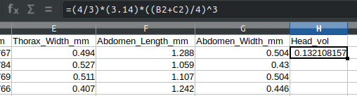
Figure 3.5: Dataset of wasp morphological measurements from five species of fig wasps collected from Baja, Mexico in 2010. Head volume (column H) has been calculated for row 2, and to calculate it for the remaining rows, the small black square in the bottom right of the highlighted cell H2 can be clicked and dragged down to H27.
Another way to achieve the same result is to copy the contents of cell H2, highlight cells H3–H27, then paste. However you do it, you should now have a new column of calculated head volumes.
Next, suppose that we want to calculate thorax and abdomen volumes for all wasps. Unlike wasp heads, wasp thoraxes and abdomens are clearly not spheres. But it is perhaps not entirely unreasonable to model them as ellipsoids. To calculate wasp thorax and abdomen volumes assuming an ellipsoid shape, we can use the formula,
\[V_{\mathrm{thorax}} = \frac{4}{3}\pi \left(\frac{Thorax_{\mathrm{L}}}{2}\right)\left(\frac{Thorax_{\mathrm{W}}}{2}\right)^{2}.\] In the equation above, \(Thorax_{\mathrm{L}}\) is thorax length (mm) and \(Thorax_{\mathrm{W}}\) is thorax width. Substitute \(Abdomen_{\mathrm{L}}\) and \(Abdomen_{\mathrm{W}}\) to instead calculate abdomen volume (\(V_{\mathrm{abdomen}}\)). What formula will you type into your empty spreadsheet cell to calculate \(V_{\mathrm{thorax}}\)? Keep in mind the order of operations indicated in the equation above.
Now fill in the columns for thorax volume and abdomen volume. You should now have three new columns of data from calculations of the volumes of the head, thorax, and abdomen of each wasp. Lastly, add one final column of data for total volume, which is the sum of the three segments.
There are a lot of potential sources of error and uncertainty in these final volumes. What are some reasons that we might want to be cautious about our calculated wasp volumes? Explain in 2–3 sentences.
Save your wasp morphology file as a CSV. This was the last exercise of the chapter. You should now be comfortable formatting tidy datasets for use in jamovi.
3.5 Summary
Completing this practical should give you the skills that you need to prepare datasets for statistical analysis.
There are many additional features of spreadsheets that were not introduced (mainly because we will do them in jamovi) but could be useful to learn.
For example, if we wanted to calculate the sum of all head lengths, we could use the function =sum(B2:B27) in any spreadsheet cell (where B2 is the head length of the first wasp, and B27 is the head length of the last wasp).
Other functions such as =count(), =min(), =max(), or =average() can be similarly used for calculations.