Chapter 22 The t-test
A t-test is a simple and widely used statistical hypothesis test that relies on the t-distribution introduced in Chapter 19. In this chapter, we will look at three types of t-tests: (1) the one sample t-test, (2) the independent samples t-test, and (3) the paired samples t-test. We will also look at non-parametric alternatives to t-tests (Wilcoxon and Mann-Whitney tests), which become relevant when the assumptions of t-tests are violated. The use of all of these tests in jamovi will be demonstrated in Chapter 23.
22.1 One sample t-test
Suppose that a biology teacher has created a new approach to teaching and wants to test whether or not their new approach results in student test scores that are higher than the reported national average of 60. This teacher should first define their null and alternative hypotheses.
- \(H_{0}\): The mean of student test scores equals 60
- \(H_{A}\): The mean of student test scores is greater than 60
Note that this is a one-sided hypothesis. The teacher is not interested in whether or not the mean test score of their students is below 60. They just want to find out if the mean test scores are greater than 60. Suppose the teacher has 10 students with the following test scores (out of 100).
49.3, 62.9, 73.7, 65.5, 69.6, 70.7, 61.5, 73.4, 61.1, 78.1The teacher can use a one sample t-test to test \(H_{0}\). The one sample t-test will test whether the sample mean of test scores (\(\bar{y} = 66.58\)) is significantly greater than the reported national average, \(\mu_{0} = 60\). How does this work? Recall from Chapter 16 that, due to the central limit theorem, the distribution of sample means (\(\bar{y}\)) will be normally distributed around the true mean \(\mu\) as sample size \(N\) increases. At low \(N\), when we need to estimate the true standard deviation (\(\sigma\)) from the sample standard deviation (\(s\)), we need to correct for a bias and use the t-distribution (see Chapter 19). The logic here is to use the t-distribution as the null distribution for \(\bar{y}\). If we subtract \(\mu_{0}\) from \(\bar{y}\), then we can centre the mean of the null distribution at 0. We can then divide by the standard error of test scores so that we can compare the deviation of \(\bar{y}\) from \(\mu_{0}\) in terms of the t-distribution. This is the same idea as calculating a z-score from Section 16.2. In fact, the equations look almost the same,
\[t_{\bar{y}} = \frac{\bar{y} - \mu_{0}}{\mathrm{SE}(\bar{y})}.\]
In the above equation, \(\mathrm{SE}(\bar{y})\) is the standard error of \(\bar{y}\).
If the sample mean of test scores is really the same as the population mean \(\mu_{0} = 60\), then \(\bar{y}\) should have a t-distribution. Consequently, values of \(t_{\bar{y}}\) far from zero would suggest that the sample mean is improbable given the null distribution predicted if \(H_{0}: \mu_{0} = \bar{y}\) is true. We can calculate \(t_{\bar{y}}\) for our above sample (note, \(\mathrm{SE}(\bar{y}) = s/\sqrt{N} = 8.334373 / \sqrt{10} = 2.63556\)),
\[t_{\bar{y}} = \frac{66.58 - 60}{2.63556} = 2.496623.\]
Our t-statistic is therefore 2.496623 (note that a t-statistic can also be negative; this would just mean that our sample mean is less than \(\mu_{0}\), instead of greater than \(\mu_{0}\), but nothing about the t-test changes if this is the case). We can see where this value falls on the t-distribution with 9 degrees of freedom in Figure 22.1.
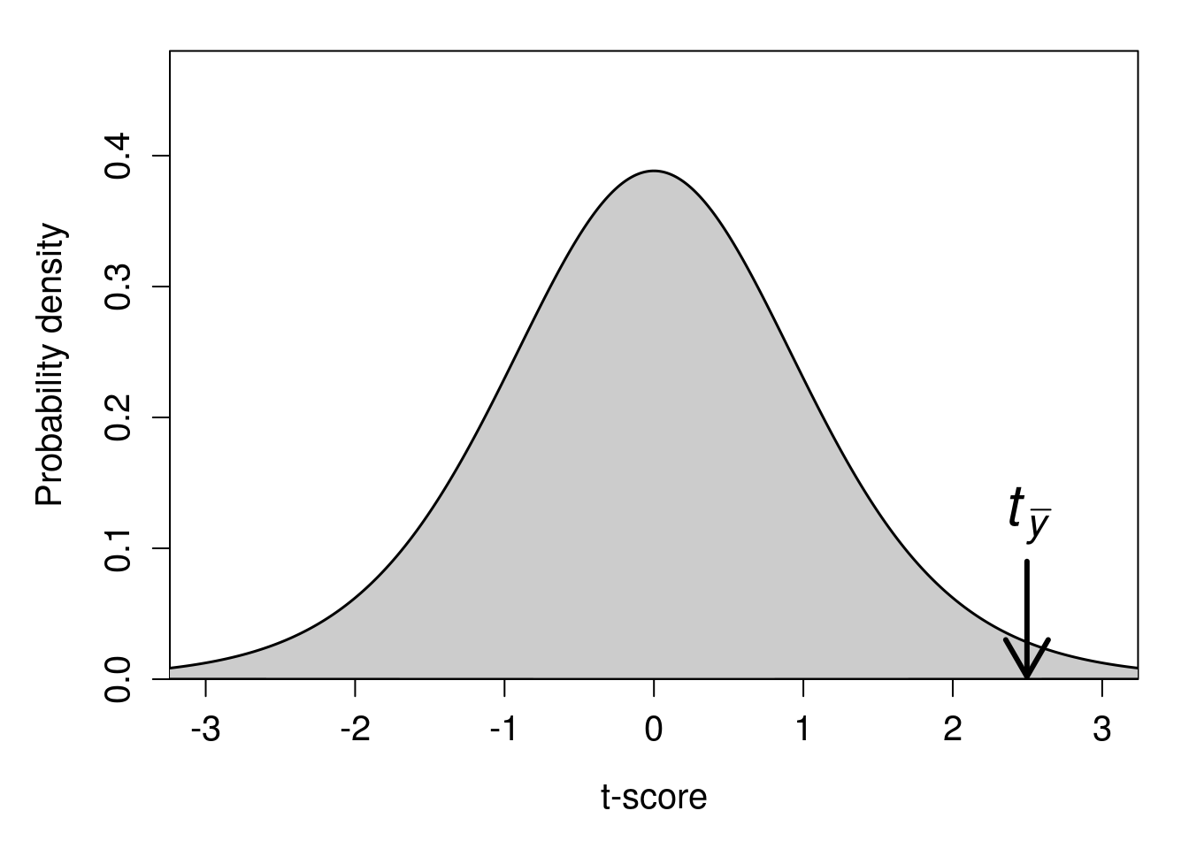
Figure 22.1: A t-distribution is shown with a calculated t-statistic of 2.49556 indicated with a downward arrow.
The t-distribution in Figure 22.1 is the probability distribution if \(H_{0}\) is true (i.e., the student test scores were sampled from a distribution with a mean of \(\mu_{0} = 60\)). The arrow pointing to the calculated \(t_{\bar{y}} = 2.496623\) indicates that if \(H_{0}\) is true, then the sample mean of student test scores \(\bar{y} = 66.58\) would be very unlikely. This is because only a small proportion of the probability distribution in Figure 22.1 is greater than or equal to our t-statistic, \(t_{\bar{y}} = 2.496623\). In fact, the proportion of t-statistics greater than 2.496623 is only about \(P =\) 0.017. Hence, if our null hypothesis is true, then the probability of getting a mean student test score of 66.58 or higher is \(P =\) 0.017 (this is our p-value). It is important to understand the relationship between the t-statistic and the p-value; an interactive application45 can help visualise. Typically, we set a threshold level of \(\alpha = 0.05\), below which we conclude that our p-value is statistically significant (see Chapter 21). Consequently, because our p-value is less than 0.05, we reject our null hypothesis and conclude that student test scores are higher than the reported national average.
22.2 Independent samples t-test
Perhaps the biology teacher is not actually interested in comparing their students’ test results with those of the reported national average. After all, there might be many reasons their students score differently from the national average that have nothing to do with their new approach to teaching. To see if their new approach is working, the teacher might instead decide that a better hypothesis to test is whether or not the mean test score from the current year is higher than the mean test score from the class that they taught in the previous year. We can use \(\bar{y}_{1}\) to denote the mean of test scores from the current year, and \(\bar{y}_{2}\) to denote the mean of test scores from the previous year. The test scores of the current year (\(y_{1}\)) therefore remain the same as in the example of the one sample t-test from the previous section.
49.3, 62.9, 73.7, 65.5, 69.6, 70.7, 61.5, 73.4, 61.1, 78.1Suppose that in the previous year, there were 9 students in the class (i.e., one fewer than the current year). These 9 students received the following test scores (\(y_{2}\)).
57.4, 52.4, 70.5, 71.6, 46.1, 60.4, 70.0, 64.5, 58.8The mean score from last year was \(\bar{y}_{2} = 61.30\), which does appear to be lower than the mean score of the current year, \(\bar{y}_{1} = 66.58\). But is the difference between these two means statistically significant? In other words, were the test scores from each year sampled from a population with the same mean, such that the population mean of the previous year (\(\mu_{2}\)) and the current year (\(\mu_{1}\)) are the same? This is the null hypothesis, \(H_{0}: \mu_{1} = \mu_{2}\).
The general idea for testing this null hypothesis is the same as it was in the one sample t-test. In both cases, we want to calculate a t-statistic, then see where it falls along the t-distribution to decide whether or not to reject \(H_{0}\). In this case, our t-statistic (\(t_{\bar{y}_{1} - \bar{y}_{2}}\)) is calculated slightly differently,
\[t_{\bar{y}_{1} - \bar{y}_{2}} = \frac{\bar{y}_{1} - \bar{y}_{2}}{\mathrm{SE}(\bar{y})}\]
The logic is the same as the one sample t-test. If \(\mu_{1} = \mu_{2}\), then we also would expect \(\bar{y}_{1} = \bar{y}_{2}\) (i.e., \(\bar{y}_{1} - \bar{y}_{2} = 0\)). Differences between \(\bar{y}_{1}\) and \(\bar{y}_{2}\) cause the t-statistic to be either above or below 0, and we can map this deviation of \(t_{\bar{y}_{1} - \bar{y}_{2}}\) from 0 to the probability density of the t-distribution after standardising by the standard error (\(\mathrm{SE}(\bar{y})\)).
What is \(\mathrm{SE}(\bar{y})\) in this case? After all, there are two different samples \(y_{1}\) and \(y_{2}\), so could the two samples not have different standard errors? This could indeed be the case, and how we actually conduct the independent samples t-test depends on whether or not we are willing to assume that the two samples came from populations with the same variance (i.e., \(\sigma_{1} = \sigma_{2}\)). If we are willing to make this assumption, then we can pool the variances (\(s^{2}_{p}\)) together to get a combined (more accurate) estimate of the standard error \(\mathrm{SE}(\bar{y})\) from both samples46\(^{,}\)47. This version of the independent samples t-test is called the ‘Student’s t-test’.
If we are unwilling to assume that \(y_{1}\) and \(y_{2}\) have the same variance, then we need to use an alternative version of the independent samples t-test. This alternative version is called the Welch’s t-test (Welch, 1938), also known as the unequal variances t-test (Dytham, 2011; Ruxton, 2006). In contrast to the Student’s t-test, the Welch’s t-test does not pool the variances of the samples together48. While there are some mathematical differences between the Student’s and Welch’s independent samples t-tests, the general concept is the same.
This raises the question, when is it acceptable to assume that \(y_{1}\) and \(y_{2}\) have the same variance? The sample variance of \(s^{2}_{1} = 69.46\) and \(s^{2}_{2} = 76.15\). Is this close enough to treat them as the same? Like a lot of choices in statistics, there is no clear right or wrong answer. In theory, if both samples do come from a population with the same variance (\(\sigma^{2}_{1} = \sigma^{2}_{2}\)), then the pooled variance is better because it gives us a bit more statistical power; we can correctly reject the null hypothesis more often when it is actually false (i.e., it decreases the probability of a Type II error). Nevertheless, the increase in statistical power is quite low, and the risk of pooling the variances when they actually are not the same increases the risk that we reject the null hypothesis when it is actually true (i.e., it increases the probability of a Type I error, which we definitely do not want!). For this reason, some researchers advocate using the Welch’s t-test by default, unless there is a very good reason to believe \(y_{1}\) and \(y_{2}\) are sampled from populations with the same variance (Delacre et al., 2017; Ruxton, 2006).
Here we will adopt the traditional approach of first testing the null hypothesis that \(\sigma^{2}_{1} = \sigma^{2}_{2}\) using a homogeneity of variances test. If we fail to reject this null hypothesis (i.e., \(P > 0.05\)), then we will use the Student’s t-test, and if we reject it (i.e., \(P < 0.05\)), then we will use the Welch’s t-test. This approach is mostly used for pedagogical reasons; in practice, defaulting to the Welch’s t-test is fine (Delacre et al., 2017; Ruxton, 2006). Testing for homogeneity of variances is quite straightforward in most statistical programs, and we will save the conceptual and mathematical details of this for when we look at the F-distribution in Chapter 24. But the general idea is that if \(\sigma^{2}_{1} = \sigma^{2}_{2}\), then the ratio of variances (\(\sigma^{2}_{1}/\sigma^{2}_{2}\)) has its own null distribution (like the normal distribution, or the t-distribution), and we can see the probability of getting a deviation of \(\sigma^{2}_{1}/\sigma^{2}_{2}\) from 1 if \(\sigma^{2}_{1} = \sigma^{2}_{2}\) is true.
In the case of the test scores from the two samples of students (\(y_{1}\) and \(y_{2}\)), a homogeneity of variance test reveals no evidence that \(s^{2}_{1} = 69.46\) and \(s^{2}_{2} = 76.15\) are significantly different (\(P = 0.834\)). We can therefore use the pooled variance and the Student’s independent samples t-test. We can calculate \(\mathrm{SE}(\bar{y}) = 3.915144\) using the formula for \(s_{p}\) (again, this is not something that ever actually needs to be done by hand), then find \(t_{\bar{y}_{1} - \bar{y}_{2}}\),
\[t_{\bar{y}_{1} - \bar{y}_{2}} = \frac{\bar{y}_{1} - \bar{y}_{2}}{\mathrm{SE}(\bar{y})} = \frac{66.58 - 61.3}{3.915144} = 1.348609.\]
As with the one-sample t-test, we can identify the position of \(t_{\bar{y}_{1} - \bar{y}_{2}}\) on the t-distribution (Figure 22.2).
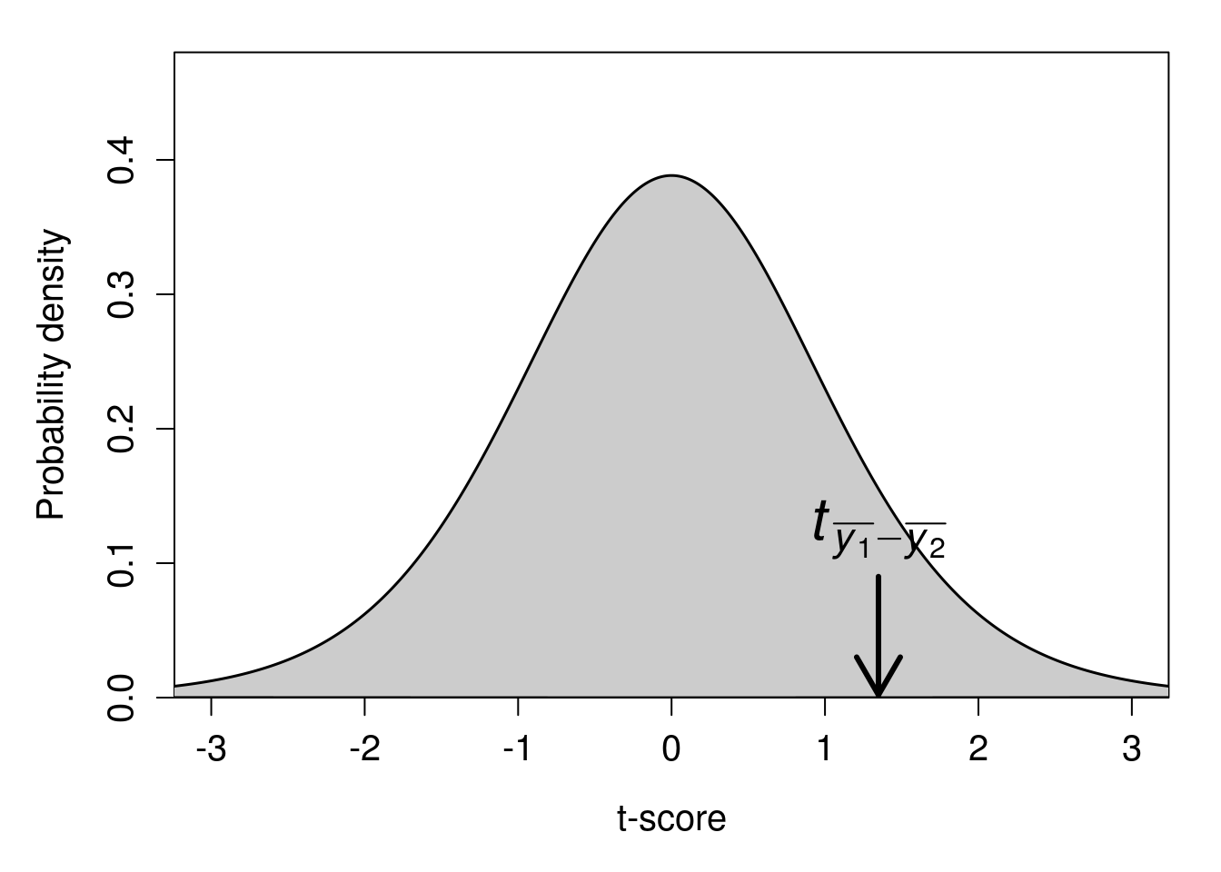
Figure 22.2: A t-distribution is shown with a calculated t-statistic of 1.348609 indicated with a downward arrow.
The proportion of t-scores that are higher than \(t_{\bar{y}_{1} - \bar{y}_{2}} = 1.348609\) is about 0.098. In other words, given that the null hypothesis is true, the probability of getting a t-statistic this high is \(P = 0.098\). Because this p-value exceeds our critical value of \(\alpha = 0.05\), we do not reject the null hypothesis. We therefore should conclude that the mean of test scores from the current year (\(\bar{y}_{1}\)) is not significantly different from the mean of test scores in the previous year (\(\bar{y}_{2}\)). The biology teacher in our example might therefore conclude that mean test results have not improved from the previous year.
22.3 Paired samples t-test
There is one more type of t-test to consider. The paired samples t-test is applied when the data points in one sample can be naturally paired with those in another sample. In this case, data points between samples are not independent. For example, we can consider the student test scores (\(y_{1}\)) yet again.
49.3, 62.9, 73.7, 65.5, 69.6, 70.7, 61.5, 73.4, 61.1, 78.1Suppose that the teacher gave these same 10 students (S1–S10) a second test and wanted to see if the mean student score changed from one test to the next (i.e., a two-sided hypothesis).
| S1 | S2 | S3 | S4 | S5 | S6 | S7 | S8 | S9 | S10 | |
|---|---|---|---|---|---|---|---|---|---|---|
| Test 1 | 49.3 | 62.9 | 73.7 | 65.5 | 69.6 | 70.7 | 61.5 | 73.4 | 61.1 | 78.1 |
| Test 2 | 46.6 | 62.7 | 73.8 | 58.3 | 66.8 | 69.7 | 64.5 | 71.3 | 64.5 | 78.8 |
| Change | -2.7 | -0.2 | 0.1 | -7.2 | -2.8 | -1 | 3 | -2.1 | 3.4 | 0.7 |
In this case, what we are really interested in is the change in scores from Test 1 to Test 2. We want to test the null hypothesis that this change is zero. This is actually the same test as the one-sample t-test. We are just substituting the mean difference in values (i.e., ‘Change’ in Table 22.1) for \(\bar{y}\) and setting \(\mu_{0} = 0\). We can calculate \(\bar{y} = -0.88\) and \(\mathrm{SE}(\bar{y})=0.9760237\), then set up the t-test as before,
\[t_{\bar{y}} = \frac{-0.88 - 0}{0.9760237} = -0.9016175.\]
Again, we can find the location of our t-statistic \(t_{\bar{y}} = -0.9016175\) on the t-distribution (Figure 22.3).
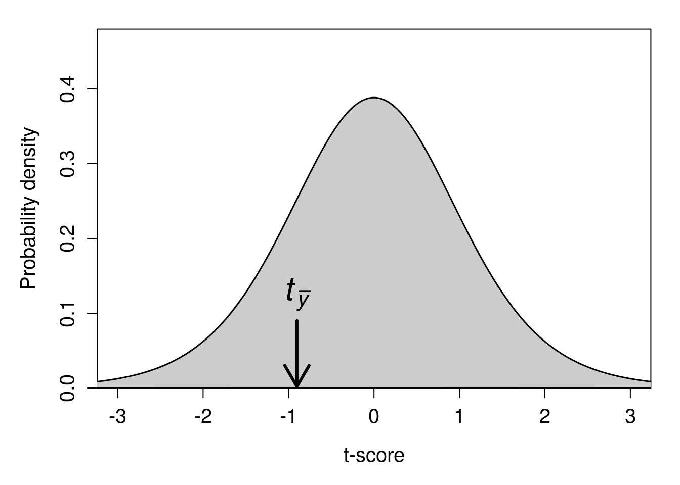
Figure 22.3: A t-distribution is shown with a calculated t-statistic of \(-0.9016175\) indicated with a downward arrow.
Since this is a two-sided hypothesis, we want to know the probability of getting a t-statistic as extreme as \(-0.9016175\) (i.e., either \(\pm 0.9016175\)) given that the null distribution is true. In the above t-distribution, 95% of the probability density lies between \(t = -2.26\) and \(t = 2.26\). Consequently, our calculated \(t_{\bar{y}} = -0.9016175\) is not sufficiently extreme to reject the null hypothesis. The p-value associated with \(t_{\bar{y}} = -0.9016175\) is \(P = 0.391\). We therefore fail to reject \(H_{0}\) and conclude that there is no significant difference in student test scores from Test 1 to Test 2.
22.4 Assumptions of t-tests
We make some potentially important assumptions when using t-tests. A consequence of violating these assumptions is a misleading Type I error rate. That is, if our data do not fit the assumptions of our statistical test, then we might not actually be rejecting our null hypothesis at the \(\alpha = 0.05\) level. We might unknowingly be rejecting \(H_{0}\) when it is true at a much higher \(\alpha\) value, and therefore concluding that we have evidence supporting the alternative hypothesis \(H_{A}\) when we really do not. It is important to recognise the assumptions that we are making when using any statistical test (including t-tests). If our assumptions are violated, we might need to use a different test, or perhaps apply some kind of transformation on the data. Assumptions that we make when conducting a t-test are as follows:
- Data are continuous (i.e., not count or categorical data)
- Sample observations are a random sample from the population
- Sample means are normally distributed around the true mean
Note that if we are running a Student’s independent samples t-test that pools sample variances (rather than a Welch’s t-test), then we are also assuming that sample variances are the same (i.e., homogeneity of variance). The last bullet point concerning normally distributed sample means is frequently misunderstood to mean that the sample data themselves need to be normally distributed. This is not the case (Johnson, 1995; Lumley et al., 2002). Instead, what we are really concerned with is the distribution of sample means (\(\bar{y}\)) around the true mean (\(\mu\)). And given a sufficiently large sample size, a normal distribution is assured due to the central limit theorem (see Chapter 16).
Moreover, while a normally distributed variable is not necessary for satisfying the assumptions of a t-test (or many other tests introduced in this book), it is sufficient. In other words, if the variable being measured is normally distributed, then the sample means will also be normally distributed around the true mean (even for a low sample size). So when is a sample size large enough, or close enough to being normally distributed, for the assumption of normality to be satisfied? There really is not a definitive answer to this question, and the truth is that most statisticians will prefer to use a histogram (or some other visualisation approach) and their best judgement to decide if the assumption of normality is likely to be violated.
This book will take the traditional approach of running a statistical test called the Shapiro-Wilk test to test the null hypothesis that data are normally distributed. If we reject the null hypothesis (when \(P < 0.05\)), then we will conclude that the assumption of normality is violated, and the t-test is not appropriate. The details of how the Shapiro-Wilk test works are not important for now, but the test can be easily run using jamovi (The jamovi project, 2024). If we reject the null hypothesis that the data are normally distributed, then we can use one of two methods to run our statistical test.
- Transform the data in some way (e.g., take the log of all values) to improve normality.
- Use a non-parametric alternative test.
The word ‘non-parametric’ in this context just means that there are no assumptions (or very few) about the shape of the distribution (Dytham, 2011). We will consider the non-parametric equivalents of the one-sample t-test (the Wilcoxon test) and independent samples t-test (Mann-Whitney U test) in the next section. But first, we can show how transformations can be used to improve the fit of the data to satisfy model assumptions.
Often data will have a skewed distribution (see Chapter 13). For example, in Figure 22.4A, we have a dataset (sample size \(N = 200\)) with a large positive skew (i.e., it is right-skewed). Most values are in the same general area, but with some values being especially high.
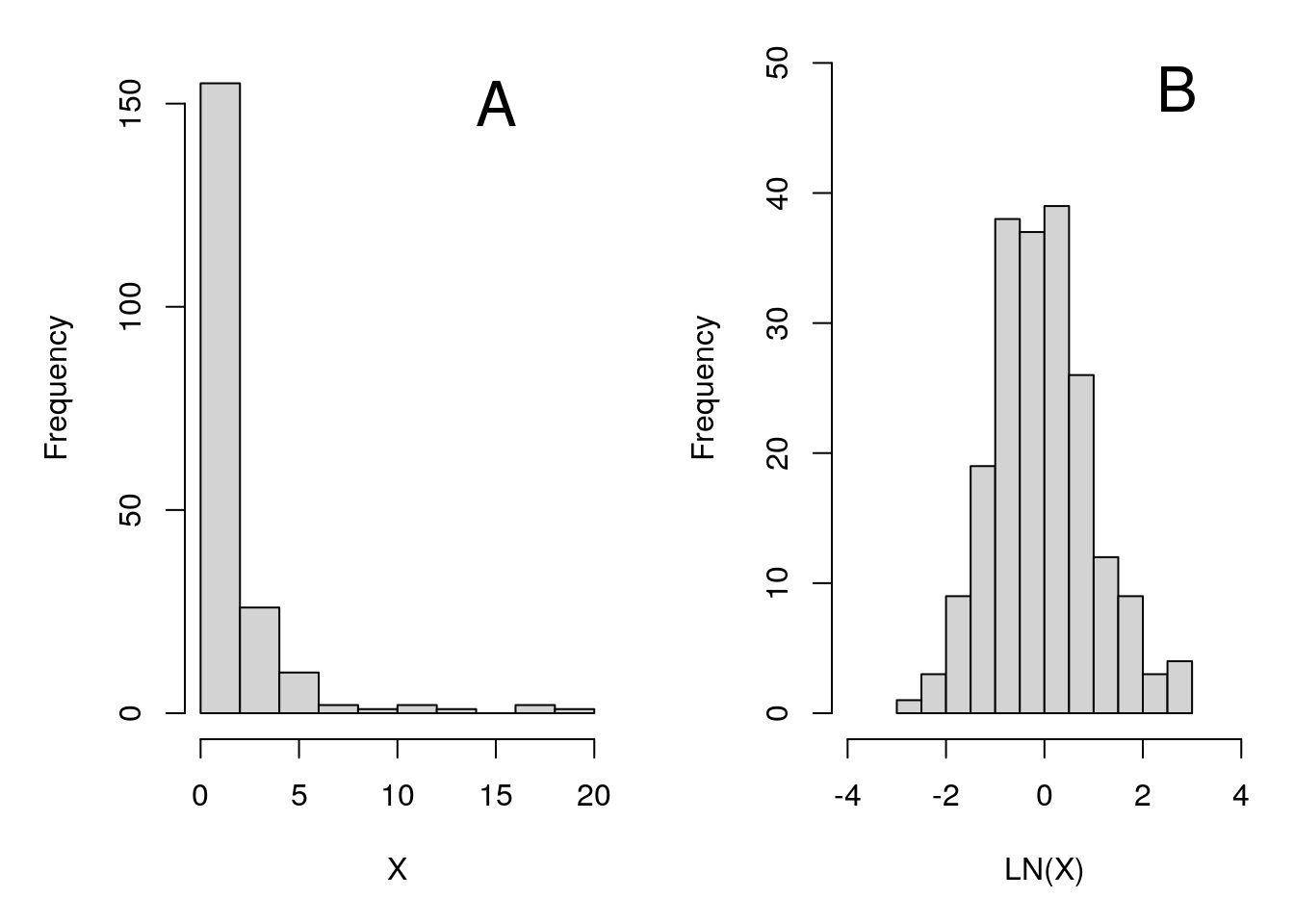
Figure 22.4: Set of values with a high positive skew (A), which, when log-transformed (i.e., when we take the natural log of all values), have a normal distribution (B).
Using a t-test on the variable \(X\) shown in Figure 22.4A is probably not a good idea. But taking the natural log of all the values of \(X\) makes the dataset more normally distributed (Figure 22.4B), thereby more convincingly satisfying the normality assumption required by the t-test. This might seem a bit suspicious at first. Is it really okay to just take the logarithm of all the data instead of the actual values that were measured? Actually, there is no real scientific or statistical reason that we need to use the original scale (Sokal & Rohlf, 1995). Using the log or the square-root of a set of numbers is perfectly fine if it helps satisfy the assumptions of a statistical test.
22.5 Non-parametric alternatives
If we find that the assumption of normality is not satisfied, and a transformation of the data cannot help, then we can consider using non-parametric alternatives to a t-test. These alternatives include the Wilcoxon test and the Mann-Whitney U test.
22.5.1 Wilcoxon test
The Wilcoxon test (also called the ‘Wilcoxon signed-rank test’) is the non-parametric alternative to a one sample t-test (or a paired t-test). Instead of using the actual data, the Wilcoxon test ranks all of the values in the dataset, then sums up their signs (either positive or negative). The general idea is that we can compare the sum of the ranks of the actual data with what would be predicted by the null hypothesis. It tests the null hypothesis that the median (\(M\)) is significantly different from some given value49. An example will make it easier to see how it works. We can use the same hypothetical dataset on student test scores.
49.3, 62.9, 73.7, 65.5, 69.6, 70.7, 61.5, 73.4, 61.1, 78.1The first step is to subtract the null hypothesis value (\(M = 60\), if we again set \(H_{0}\) to be that the average student test score equals 60) from each value (\(49.3 - 60 = -10.7\), \(62.9 - 60 = 2.9\), etc.).
-10.7, 2.9, 13.7, 5.5, 9.6, 10.7, 1.5, 13.4, 1.1, 18.1We need to note the sign of each value as negative (\(-\)) or positive (\(+\)).
-, +, +, +, +, +, +, +, +, +Next, we need to compute the absolute values of the numbers (i.e., \(|-10.7| = 10.7\), \(|2.9| = 2.9\), \(|13.7| = 13.7\), etc.).
10.7, 2.9, 13.7, 5.5, 9.6, 10.7, 1.5, 13.4, 1.1, 18.1We then rank these values from lowest to highest and record the sign of each value.
6.5, 3.0, 9.0, 4.0, 5.0, 6.5, 2.0, 8.0, 1.0, 10.0Note that both the first and sixth position had the same value (10.7), so instead of ranking them as 6 and 7, we split the difference and rank both as 6.5. Now, we can calculate the sum of the negative ranks (\(W^{-}\)), and the positive ranks \(W^{+}\). In this case, the negative ranks are easy; there is only one value (the first one), so the sum is just 6.5,
\[W^{-} = 6.5\]
The positive ranks are in positions 2–10, and the rank values in these positions are 3, 9, 4, 5, 6.5, 2, 8, 1, and 10. The sum of our positive ranks is therefore,
\[W^{+} = 3.0 + 9.0 + 4.0 + 5.0 + 6.5 + 2.0 + 8.0 + 1.0 + 10.0 = 48.5\]
Note that \(W^{-}\) plus \(W^{+}\) (i.e., 6.5 + 48.5 = 55 in the example here) will always be the same for a given sample size \(N\) (in this case, \(N = 10\)),
\[W = \frac{N \left(N + 1 \right)}{2}.\]
What the Wilcoxon test is doing is calculating the probability of getting a value of \(W^{+}\) as or more extreme than would be the case if the null hypothesis is true. Note that if, e.g., there are an equal number of values above and below the median, then both \(W^{-}\) and \(W^{+}\) will be relatively low and about the same value. This is because the ranks of the values below 0 (which we multiply by \(-1\)) and above 0 (which we multiply by 1) will be about the same. But if there are a lot more values above the median than expected (as with the example above), then \(W^{+}\) will be relatively high. And if there are a lot more values below the median than expected, then \(W^{+}\) will be relatively low.
To find the probability of \(W^{+}\) being as low or high as it is given that the null hypothesis is true (i.e., the p-value), we need to compare the test statistic \(W^{+}\) to its distribution under the null hypothesis (note that we can also conduct a one-tailed hypothesis, in which case we are testing if \(W^{+}\) is either higher or lower than expected given \(H_{0}\)). The old way of doing this is to compare the calculated \(W^{+}\) to threshold values from a Wilcoxon Signed-Ranks Table. This critical value table is no longer necessary, and statistical software such as jamovi will calculate a p-value for us. For the example above, the p-value associated with \(W^{+} = 48.5\) and \(N = 10\) is \(P = 0.037\). Since this p-value is less than our threshold of \(\alpha = 0.05\), we can reject the null hypothesis and conclude that the median of our dataset is significantly different from 60.
Note that we can also use a Wilcoxon signed rank test as a non-parametric equivalent to a paired t-test. In this case, instead of subtracting out the null hypothesis of our median value (e.g., \(H_{0}: M = 60\) in the example above), we just need to subtract the paired values. Consider again the example of the two different tests introduced for the paired samples t-test above (Table 22.2).
| S1 | S2 | S3 | S4 | S5 | S6 | S7 | S8 | S9 | S10 | |
|---|---|---|---|---|---|---|---|---|---|---|
| Test 1 | 49.3 | 62.9 | 73.7 | 65.5 | 69.6 | 70.7 | 61.5 | 73.4 | 61.1 | 78.1 |
| Test 2 | 46.6 | 62.7 | 73.8 | 58.3 | 66.8 | 69.7 | 64.5 | 71.3 | 64.5 | 78.8 |
| Change | -2.7 | -0.2 | 0.1 | -7.2 | -2.8 | -1 | 3 | -2.1 | 3.4 | 0.7 |
If the ‘Change’ values in Table 22.2 were not normally distributed, then we could apply a Wilcoxon test to test the null hypothesis that the median value of \(Test\:2 - Test\:1 = 0\) (note that a Shapiro-Wilk normality test does not reject the null hypothesis that the difference between test scores is normally distributed, so the paired t-test would be preferred in this case). To do this, we would first note the sign of each value as negative or positive.
-, -, +, -, -, -, +, -, +, +Next, we would rank the absolute values of the changes.
6, 2, 1, 10, 7, 4, 8, 5, 9, 3If we then sum the ranks, we get \(W^{-} = 6 + 2 + 10 + 7 + 4 + 5 = 34\) and \(W^{+} = 1 + 8 + 9 + 3 = 21\). The p-value associated with \(W^{+} = 21\) and \(N = 10\) in a two-tailed test is \(P = 0.557\), so we do not reject the null hypothesis that Test 1 and Test 2 have the same median.
22.5.2 Mann-Whitney U test
A non-parametric alternative to the independent samples t-test is the Mann-Whitney U test. That is, a Mann-Whitney U test can be used if we want to know whether the median of two independent groups is significantly different. Like the Wilcoxon test, the Mann-Whitney U test uses the ranks of values rather than the values themselves. In the Mann-Whitney U test, the general idea is to rank all of the data across both groups, then see if the sum of the ranks is significantly different (Fryer, 1966; Sokal & Rohlf, 1995). To demonstrate this, we can again consider the same hypothetical dataset used when demonstrating the independent samples t-test above. Test scores from the current year (\(y_{1}\)) are below.
49.3, 62.9, 73.7, 65.5, 69.6, 70.7, 61.5, 73.4, 61.1, 78.1We want to know if the median of the above scores is significantly different from the median scores in the previous year (\(y_{2}\)) shown below.
57.4, 52.4, 70.5, 71.6, 46.1, 60.4, 70.0, 64.5, 58.8There are 19 values in total, 10 values for \(y_{1}\) and 9 values for \(y_{2}\). We therefore rank all of the above values from 1 to 19. For \(y_{1}\), the ranks are below.
2, 9, 18, 11, 12, 15, 8, 17, 7, 19For \(y_{2}\), the ranks are below.
4, 3, 14, 16, 1, 6, 13, 10, 5This might be easier to see if we present it as a table showing the test Year (\(y_{1}\) versus \(y_{2}\)), test Score, and test Rank (Table 22.3).
| Year | Score | Rank |
|---|---|---|
| 1 | 49.3 | 2 |
| 1 | 62.9 | 9 |
| 1 | 73.7 | 18 |
| 1 | 65.5 | 11 |
| 1 | 69.6 | 12 |
| 1 | 70.7 | 15 |
| 1 | 61.5 | 8 |
| 1 | 73.4 | 17 |
| 1 | 61.1 | 7 |
| 1 | 78.1 | 19 |
| 2 | 57.4 | 4 |
| 2 | 52.4 | 3 |
| 2 | 70.5 | 14 |
| 2 | 71.6 | 16 |
| 2 | 46.1 | 1 |
| 2 | 60.4 | 6 |
| 2 | 70 | 13 |
| 2 | 64.5 | 10 |
| 2 | 58.8 | 5 |
What we need to do now is sum the ranks for \(y_{1}\) and \(y_{2}\). If we add up the \(y_{1}\) ranks, then we get a value of \(R_{1}=\) 118. If we add up the \(y_{2}\) ranks, then we get a value of \(R_{2}=\) 72. We can then calculate a value \(U_{1}\) from \(R_{1}\) and the sample size of \(y_{1}\) (\(N_{1}\)),
\[U_{1} = R_{1} - \frac{N_{1}\left(N_{1} + 1 \right)}{2}.\]
In the case of our example, \(R_{1}=\) 118 and \(N_{1} = 10\). We therefore calculate \(U_{1}\),
\[U_{1} = 118 - \frac{10\left(10 + 1 \right)}{2} = 63.\]
We then calculate \(U_{2}\) using the same general formula,
\[U_{2} = R_{2} - \frac{N_{2}\left(N_{2} + 1 \right)}{2}.\]
From the above example of test scores,
\[U_{2} = 72 - \frac{9\left(9 + 1 \right)}{2} = 27.\]
Whichever of \(U_{1}\) or \(U_{2}\) is lower50 is set to \(U\), so for our example, \(U = 27\). Note that if \(y_{1}\) and \(y_{2}\) have similar medians, then \(U\) will be relatively high. But if \(y_{1}\) and \(y_{2}\) have much different medians, then \(U\) will be relatively low. One way to think about this is that if \(y_{1}\) and \(y_{2}\) are very different, then one of the two samples should have very low ranks, and the other should have very high ranks (Sokal & Rohlf, 1995). But if \(y_{1}\) and \(y_{2}\) are very similar, then their summed ranks should be nearly the same. Hence, if the deviation of \(U\) is greater than what is predicted given the null hypothesis in which the distributions (and therefore the medians) of \(y_{1}\) and \(y_{2}\) are identical, then we can reject \(H_{0}\).
As with the Wilcoxon test, we could compare our \(U\) test statistic to a critical value from a table, but jamovi will also just give us the test statistic \(U\) and associated p-value (The jamovi project, 2024). In our example above, \(U = 27\), \(N_{1} = 10\), and \(N_{2} = 9\) has a p-value of \(P = 0.156\), so we do not reject the null hypothesis. We therefore conclude that there is no evidence that there is a difference in the median test scores between the two years.
22.6 Summary
The main focus of this chapter was to provide a conceptual explanation of different statistical tests. In practice, running these tests is relatively straightforward in jamovi (this is good, as long as the tests are understood and interpreted correctly). In general, the first step in approaching these tests is to determine if the data call for a one sample test, an independent samples test, or a paired samples test. In a one sample test, the objective is to test the null hypothesis that the mean (or median) equals a specific value. In an independent samples test, there are two different groups, and the objective is to test the null hypothesis that the groups have the same mean (or median). In a paired samples test, there are two groups, but individual values are naturally paired between each group, and the objective is to test the null hypothesis that the difference between paired values is zero51. If assumptions of the t-test are violated, then it might be necessary to use a data transformation or a non-parametric test such as the Wilcoxon test (in place of a one sample or paired samples t-test) or a Mann-Whitney U test (in place of an independent samples t-test).
References
This is not a calculation that needs to be done by hand anymore. Statistical software such as jamovi will calculate \(s_{p}\) automatically from a dataset (The jamovi project, 2024). For those interested, the formula that it uses to make this calculation is, \[s_{p} = \sqrt{\frac{\left(n_{1} - 1 \right) s^{2}_{y_{1}} + \left(n_{2} - 1 \right) s^{2}_{y_{2}}}{n_{1} + n_{2} - 2}}.\] This looks like a lot, but really all the equation is doing is adding the two variances (\(s^{2}_{y_{1}}\) and \(s^{2}_{y_{2}}\)) together, but weighing them by their degrees of freedom (\(n_{1} - 1\) and \(n_{2} - 1\)), so that the one with a higher sample size has more influence on the pooled standard deviation. To get \(\mathrm{SE}(\bar{y})\), we then need to multiply by the square root of \((n_{1} + n_{2})/(n_{1}n_{2})\), \[\mathrm{SE}(\bar{y}) = s_{p}\sqrt{\frac{n_{1} + n_{2}}{n_{1}n_{2}}}.\] It might be useful to try this once by hand, but only to convince yourself that it matches the t-statistic produced by jamovi.↩︎
The degrees of freedom for the t-statistic is \(df = n_{1} + n_{2} - 2\) (Sokal & Rohlf, 1995). Jamovi handles all of this automatically (The jamovi project, 2024), so we will not dwell on it here.↩︎
The equation for calculating the Welch’s t-statistic is actually a bit simpler than the Student’s t-test that uses the pooled estimate (Ruxton, 2006). Instead of using \(s_{p}\), we define our t-statistic as, \[t_{s} = \frac{\bar{y}_{1} - \bar{y}_{2}}{ \sqrt{ \frac{s^{2}_{1}}{n_{1}} + \frac{s^{2}_{2}}{n_{2}}} }.\] The degrees of freedom, however, is quite a bit messier than it is for the independent samples Student’s t-test (Sokal & Rohlf, 1995), \[v = \frac{\left(\frac{1}{n_{1}} + \frac{(s^{2}_{2} / s^{2}_{1})}{n_{2}} \right)^{2}}{\frac{1}{n^{2}_{1}\left(n_{1} - 1 \right)} + \frac{(s^{2}_{2} / s^{2}_{1})^{2}}{n^{2}_{2}\left(n_{2} - 1 \right)}}.\] Of course, jamovi will make these calculations for us, so it is not necessary to do it by hand.↩︎
Actually, the Wilcoxon signed-rank test technically tests the null hypothesis that two distributions are identical, not just that the medians are identical (Johnson, 1995; Lumley et al., 2002). Note that if one distribution has a higher variance than another, or is differently skewed, it will also affect the ranks. In other words, if we want to compare medians, then we need to assume that the distributions have the same shape (Lumley et al., 2002). Because of this, and because the central limit theorem ensures that means will be normally distributed given a sufficiently high sample size (in which case, t-test assumptions are more likely to be satisfied), some researchers suggest that non-parametric statistics such as the Wilcoxon signed rank test should be used with caution (Johnson, 1995).↩︎
Note that you could also take the higher of the two values (Sokal & Rohlf, 1995), which is what the statistical programming language R reports (R Core Team, 2022); jamovi reports the lower of the two (The jamovi project, 2024). The null distribution from which the (identical) p-value would be calculated would just be different in this case.↩︎
Note, you could also test the null hypothesis that the difference between paired values is some value other than zero, but this is quite rare in practice.↩︎