Chapter 13 Skew and kurtosis
Following measures of central tendency in Chapter 11 and measures of spread in Chapter 12, there are two more concepts that are worth briefly mentioning. Both of these concepts concern the shape of a distribution. The first concept is skew, and the second is kurtosis. This is also a good place to introduce what the word ‘moment’ refers to in the statistics.
13.1 Skew
The skew of a distribution refers to its asymmetry (Dytham, 2011; Sokal & Rohlf, 1995), which can be observed in a histogram (Figure 13.1). What we are looking for here are the sides of the distribution, also known as the ‘tails’. When the left tail sticks out as it does in Figure 13.1A, we can describe the distribution as ‘left-skewed’ or ‘negatively skewed’. When the right tail sticks out as it does in Figure 13.1B, we can describe the distribution as ‘right-skewed’ or ‘positively skewed’.
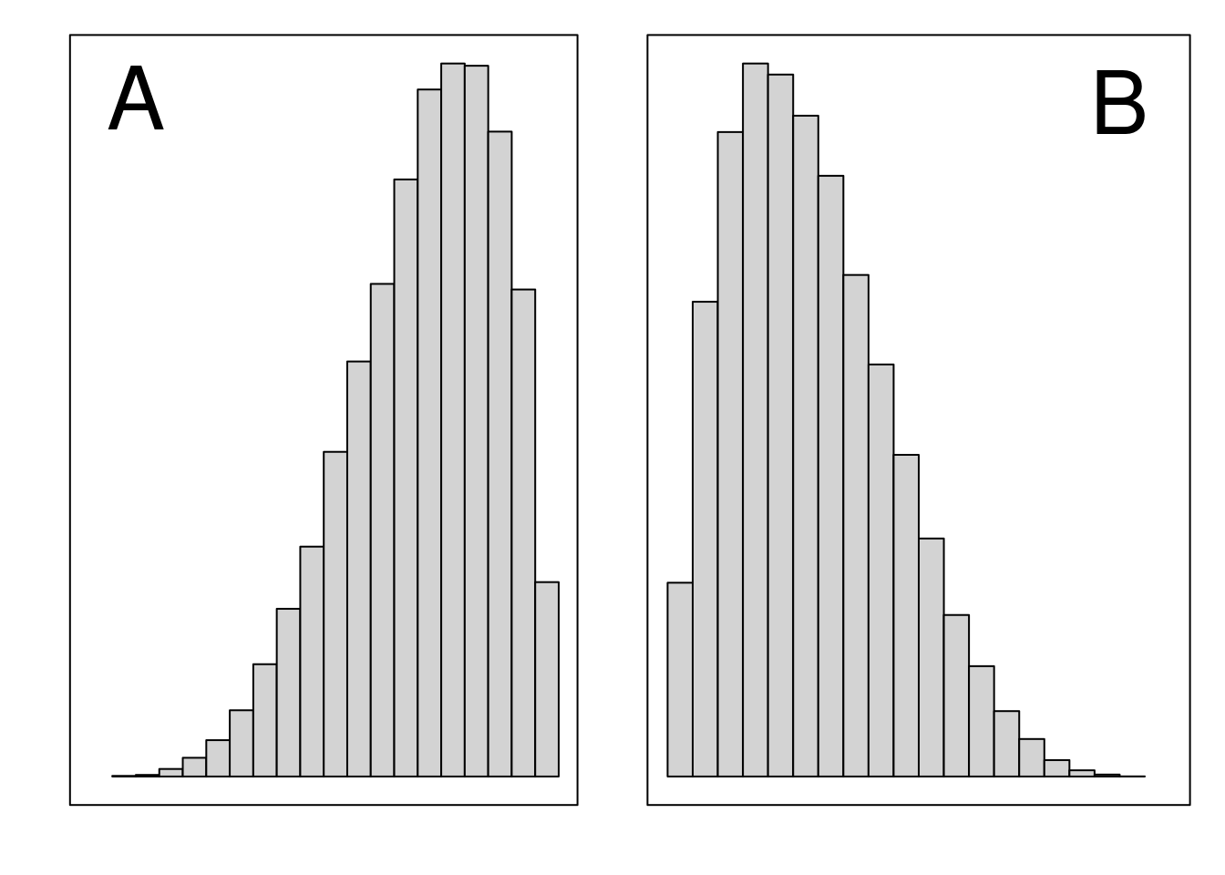
Figure 13.1: Histograms showing a (A) distribution that has a negative (i.e., ‘left’) skew and (B) distribution that has a positive (i.e., ‘right’) skew.
When a distribution is skewed, the mean and median of the distribution will be different (Sokal & Rohlf, 1995). This is because the mean of the distribution will be pulled towards the tail that sticks out due to the extreme values in the tail. In contrast, the median is robust to these extreme values. This can be important when interpreting the median versus mean as a measure of central tendency (Reichmann, 1970). For example, household income data are typically highly right-skewed because a small proportion of households have a much higher income than the typical household (McDonald et al., 2013). Consequently, when data are strongly skewed, the mean and median give us different information, and it often makes sense to use the median as an indication of what is typical (Chiripanhura, 2011).
13.2 Kurtosis
The kurtosis describes the extent to which a distribution is flat. In other words, whether data tend to be in the centre and at the tails, or whether data tend to be between the centre and tails (Sokal & Rohlf, 1995). If there are more values in the centre and tails of the distribution, then the distribution is described as ‘leptokurtic’ (Figure 13.2A). If there are more values between the centre and the tails, then the distribution is described as ‘platykurtic’ (Figure 13.2B).
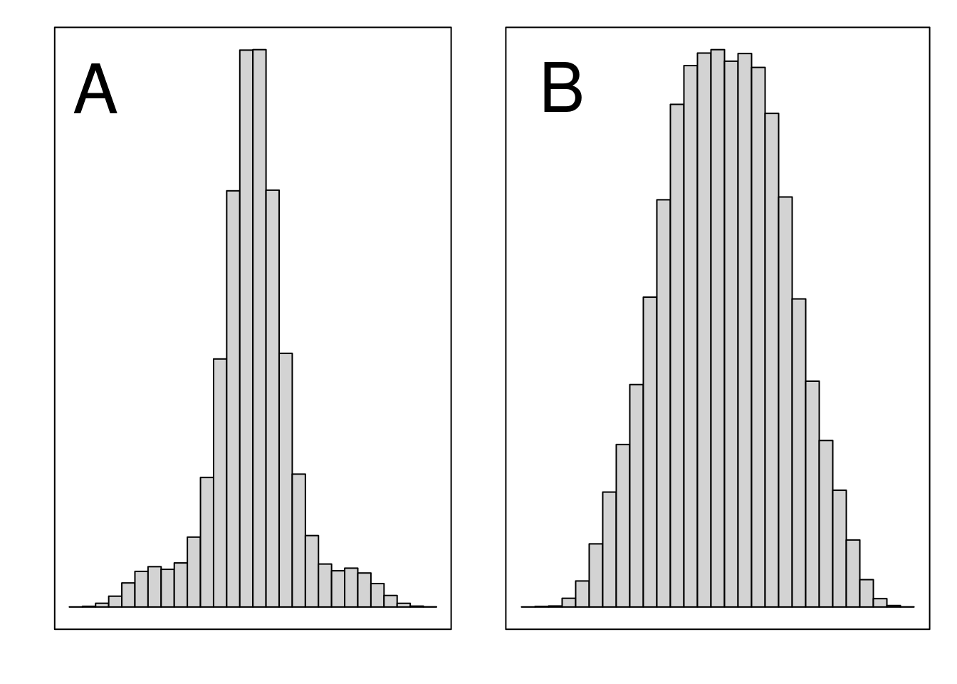
Figure 13.2: Histograms showing a (A) leptokurtic distribution and (B) platykurtic distribution.
The extent to which any given distribution is leptokurtic versus platykurtic is defined relative to the normal distribution, which will be introduced in Chapter 15.
13.3 Moments
When actually doing statistics in the biological and environmental sciences, just being able to recognise skew and kurtosis on a histogram is usually sufficient. It is possible to actually calculate skew and kurtosis as we would measures of central tendency and spread (Groeneveld & Meeden, 1984; Rahman, 1968; Sokal & Rohlf, 1995), but this is very rarely necessary (but see Doane & Seward, 2011). Nevertheless, this is a good place to introduce the concept of what a moment is in statistics.
The word ‘moment’ usually refers to a brief period in time. But this is not what the word means in statistics. In statistics, a moment is related to how much some value (more technically, a random variable) is expected to deviate from the mean (Upton & Cook, 2014). The term has its origins in physics (Miller & Miller, 2004; Sokal & Rohlf, 1995). A moment statistic describes the expected deviation from the mean, raised to some power. We have already looked at the second moment about the mean (i.e., the expected deviation raised to the power 2). This was the variance,
\[s^{2} = \frac{1}{N - 1}\sum_{i = 1}^{N}\left(x_{i} - \bar{x} \right)^{2}.\]
A different exponent would indicate a different moment. For example, a 3 would give us the third moment (skew), and a 4 would give us the fourth moment (kurtosis). The equations for calculating these sample moments are a bit more complicated than simply replacing the 2 with a 3 or 4 in the equation for variance. This is because the corrections for the third and fourth moments are no longer \(N - 1\). The corrections now also need to be scaled by the standard deviation (for details, see Sokal & Rohlf, 1995). For the purpose of doing statistics in the biological and environmental sciences, it is usually sufficient to recognise that second, third, and fourth moments refer to variance, skew, and kurtosis, respectively.