Chapter 27 Two-way ANOVA
The one-way ANOVA tested the null hypothesis that all group means are the same. But, we might also have a dataset in which there is more than one type of group. For example, suppose we know that the fig wasps used in Chapters 24–26 actually came from two different trees (Tree A and Tree B). This would mean that there could be a confounding variable affecting wing length, violating assumption 2 from Section 24.3. If, for whatever reason, fig wasps on different trees have different wing lengths, then we should include tree as an explanatory variable in the ANOVA. Because we would then have two group types (species and tree), we would need a two-way ANOVA61. Here, to illustrate the key concepts as clearly as possible, we will run an example of a two-way ANOVA with just two of the five species (Het1 and SO2). Table 27.1 shows the fig wasp wing length dataset for the two species in a tidy format, which includes columns for two group types: species and tree.
| Species | Tree | Wing Length |
|---|---|---|
| Het1 | A | 2.122 |
| Het1 | A | 1.938 |
| Het1 | B | 1.765 |
| Het1 | B | 1.700 |
| SO2 | A | 1.635 |
| SO2 | A | 1.700 |
| SO2 | B | 1.407 |
| SO2 | B | 1.378 |
We could run a one-way ANOVA (or t-test) to see if wing lengths differ between species, then run another one-way ANOVA to see if wing lengths differ between trees. But by including both group types in the same model (species and tree), we can test how one group affects wing length in the context of the other group (e.g., how tree affects wing length, while also accounting for any effects of species on wing length). We can also see if there is any synergistic effect between groups, which is called an interaction effect. For example, if Het1 fig wasps had longer wing lengths than SO2 on Tree A, but shorter wing lengths than SO2 on Tree B, then we would say that there is an interaction between species and tree. Given this kind of interaction effect, it would not make sense to say that Het1 fig wasps have longer or shorter wings than SO2 because this would depend on the tree!
This chapter will not delve into the mathematics of the two-way ANOVA62. Working out a two-way ANOVA by hand requires similar, albeit more laborious, calculations of sum of squares and degrees of freedom than is needed for the one-way ANOVA in Section 24.2. But the general concept is the same. The idea is to calculate the amount of the total variation attributable to different groups, or the interaction among group types. Note that the assumptions for the two-way ANOVA are the same as for the one-way ANOVA.
Unlike previous statistical tests in this book, we can actually test three separate null hypotheses with a two-way ANOVA. The first test is the same as the one-way ANOVA in Chapter 24, which focuses on mean species wing lengths:
- \(H_{0}:\) Mean wing lengths are the same for both species
- \(H_{A}:\) Mean wing lengths are not the same for both species
The second test focuses on the other group type, Tree:
- \(H_{0}:\) Mean wing lengths are the same in both trees
- \(H_{A}:\) Mean wing lengths are not the same in both trees
These two hypotheses address the main effects of the independent variables (species and tree) on the dependent variable (wing length). In other words, the mean effect of one group type (either species or tree) by itself, holding the other constant. The third hypothesis addresses the interaction effect:
- \(H_{0}:\) There is no interaction between species and tree
- \(H_{A}:\) There is an interaction between species and tree
Interaction effects are difficult to understand at first, so we will look at two concrete examples of two-way ANOVAs. The first will use the Table 27.1 data in which no interaction effect exists. The second will use a different species pairing in which an interaction does exist.
In a two-way ANOVA, the jamovi output (Figure 27.1) appears similar to that of a one-way ANOVA (see Section 24.2.3), but there are four rows of output. Rows 1 and 2 test the null hypotheses associated with the main effects of species and tree, respectively. Row 3 tests the interaction effect. And row 4 shows us the variation in the data that cannot be attributed to either the main effects or the interaction (i.e., residual variation). This is equivalent to the variation within groups in the one-way ANOVA.
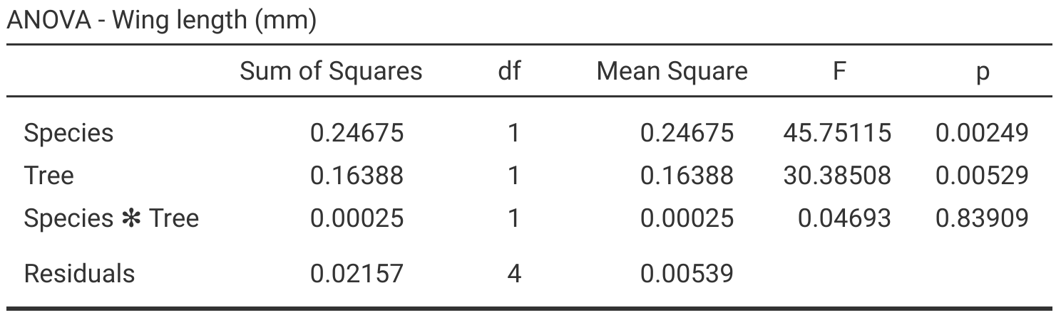
Figure 27.1: Jamovi output table for a two-way ANOVA, which tests for the effects of species (Het1 and SO2), tree, and their interaction on fig wasp wing lengths. Species wing length measurements were collected in 2010 near La Paz in Baja, Mexico.
This is a lot more information than the one-way ANOVA, but it helps to think of each row separately as a test of a different null hypothesis. From the first row, given the high \(F = 45.75\) and the low \(P = 0.002\), we can reject the null hypothesis that species mean wing lengths are the same. Similarly, from the second row, we can reject the null hypothesis that wing lengths are the same in both trees (\(F = 30.39\); \(P = 0.005\)). In contrast, from the third row, we should not reject the null hypothesis that there is no interaction between species and tree (\(F = 0.05\); \(P = 0.839\)). Figure 27.2 shows these results visually (The jamovi project, 2024).
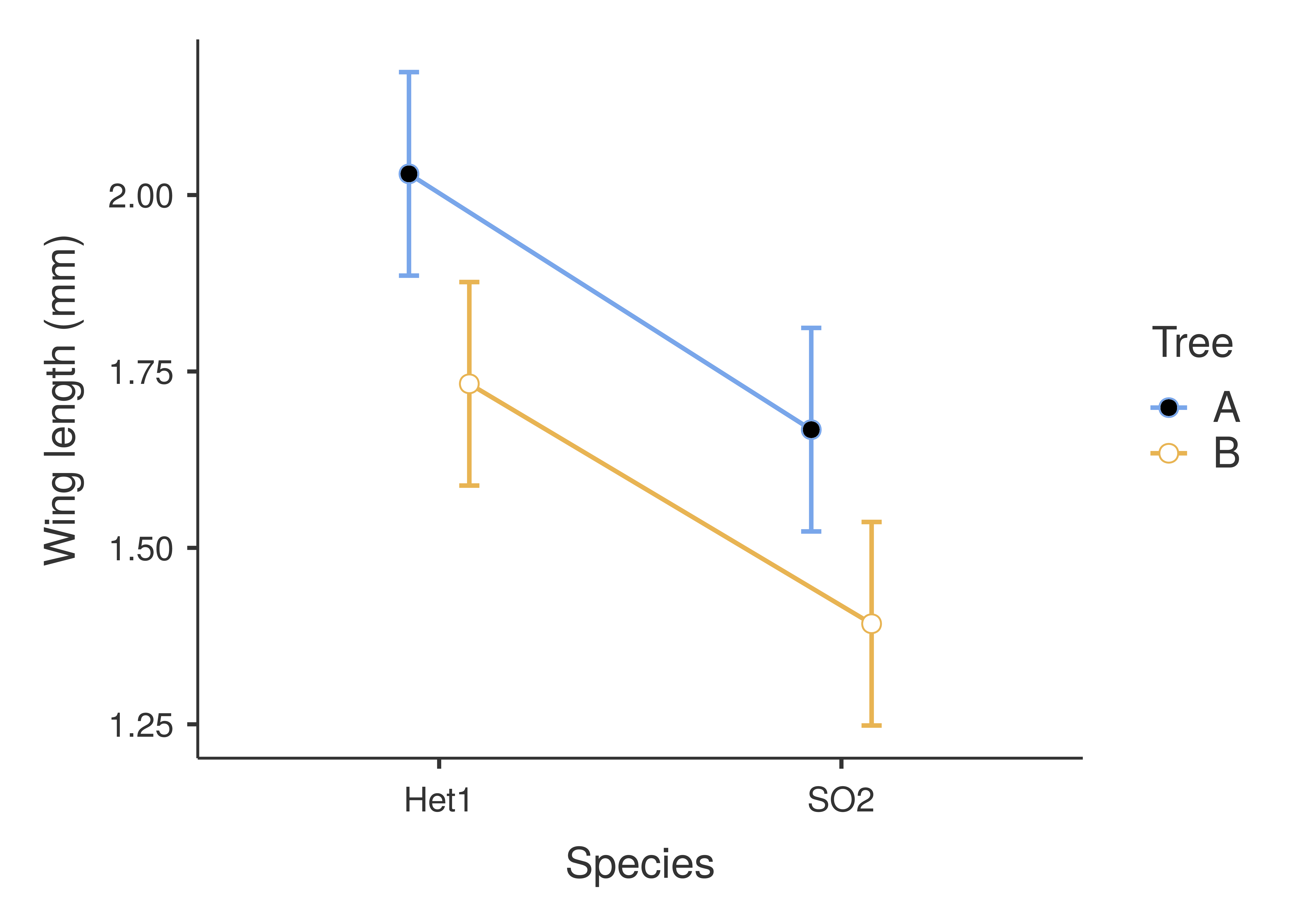
Figure 27.2: Interaction plot for a two-way ANOVA of fig wasp wing measurements as affected by species and tree. Points show mean values for the four species and tree combinations (e.g., Het1 from Tree A in the upper left). Error bars show standard errors around the means. Species wing length measurements were collected in 2010 near La Paz in Baja, Mexico.
In Figure 27.2, there is no interaction between species and tree. How can we infer this from Figure 27.2? Wing length is always consistently higher in Tree A than it is in Tree B, regardless of the species of wasp. Similarly, wing length is consistently higher for Het1 than it is for SO2, regardless of tree. Consequently, while wasp species is important for predicting wing length, as is the tree from which the wasp was collected, we do not need to consider one variable to know the effect of the other. This is reflected in the lines having a similar slope, or, more technically, slopes that are not significantly different from one another. If the slopes of the two lines were significantly different, then this would be evidence for an interaction between species and tree.
What would Figure 27.2 look like if there was an interaction effect between species and tree? We can run another two-way ANOVA, this time with a different pair of species: SO1 and SO2. Table 27.2 shows the data.
| Species | Tree | Wing Length |
|---|---|---|
| SO1 | A | 1.557 |
| SO1 | A | 1.493 |
| SO1 | B | 1.470 |
| SO1 | B | 1.541 |
| SO2 | A | 1.635 |
| SO2 | A | 1.700 |
| SO2 | B | 1.407 |
| SO2 | B | 1.378 |
If we run the two-way ANOVA in jamovi, then we can see the ANOVA output table (Figure 27.3).
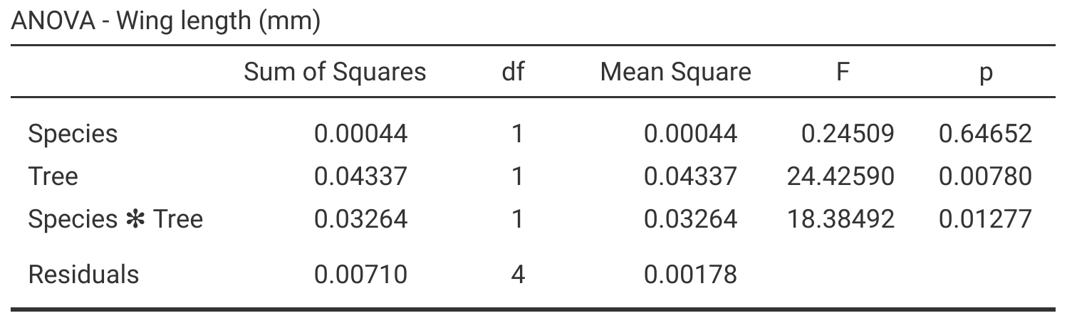
Figure 27.3: Jamovi output table for a two-way ANOVA, which tests for the effects of species (SO1 and SO2), tree, and their interaction on fig wasp wing lengths. Species wing length measurements were collected in 2010 near La Paz in Baja, Mexico.
Figure 27.3 shows that the effect of species is not significant (\(P > 0.05\)), but the effect of tree is significant (\(P < 0.05\)). Consequently, in terms of the main effects, it appears that species does not affect wing length, but tree does affect wing length. Unlike the example test between Het1 and SO2, the interaction between species and tree is significant (\(P < 0.05\)) in Figure 27.3. This means that we cannot interpret the main effects in isolation because the effect of each on wing length will change in the presence of the other. In other words, the effect of tree on wing length will depend on the species. Figure 27.4 shows this interaction visually.
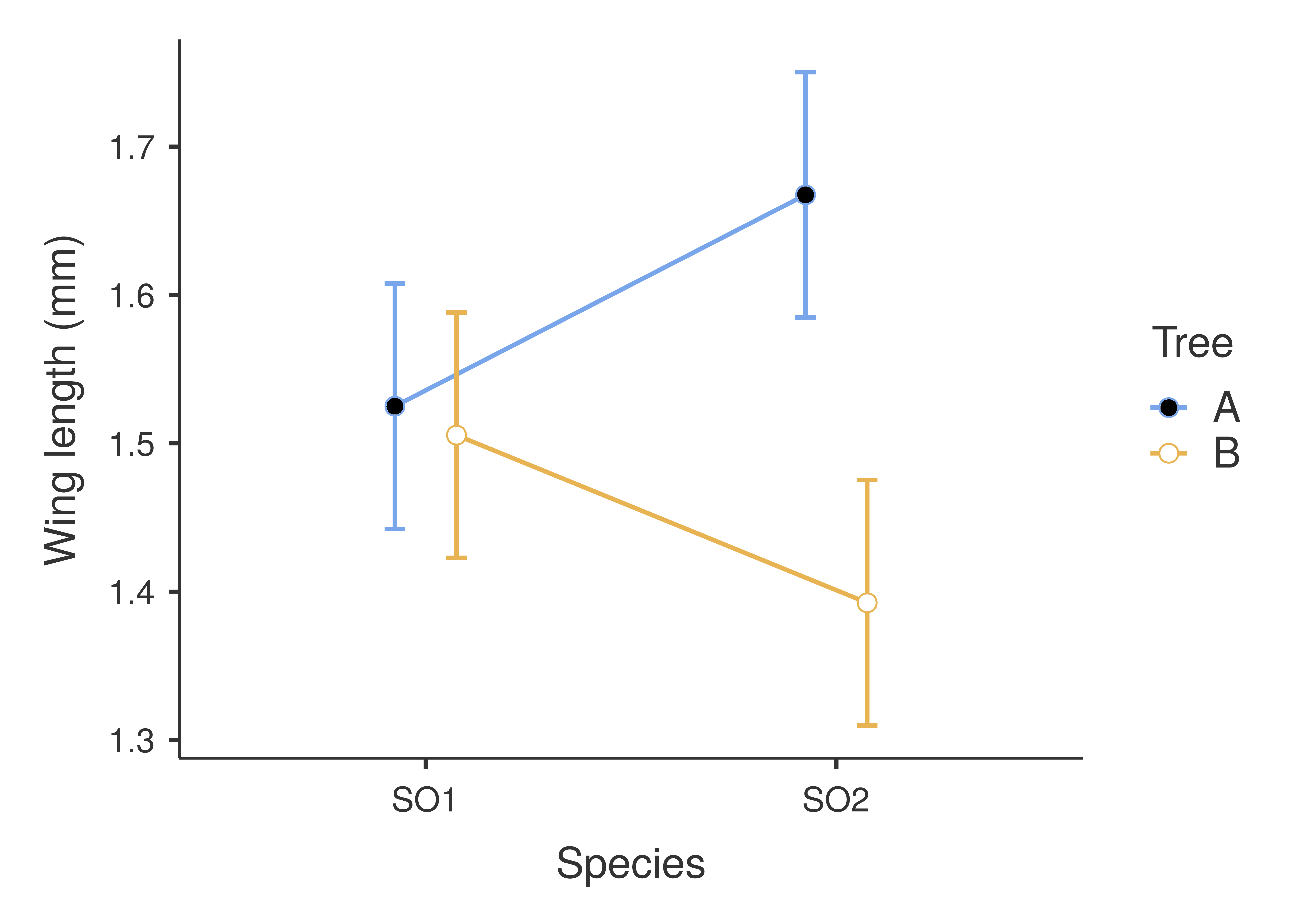
Figure 27.4: An interaction plot for a two-way ANOVA of fig wasp wing measurements as affected by species and tree. Points show mean values for the four species and tree combinations (e.g., SO2 from Tree A in the upper right). Error bars show standard errors around the means. Species wing length measurements were collected in 2010 near La Paz in Baja, Mexico.
Note that for SO1, wing length is basically the same for Trees A and B (the two left points in Figure 27.4). In contrast, for SO2, tree has a very noticeable effect on wing length! Fig wasps in species SO2 clearly have higher wing lengths on Tree A than they do on Tree B. Overall, however, the mean wing length for SO2 appears to be about the same as it is for SO1 (i.e., the middle of the two points for SO2 is at about the same wing length as it is for SO1, around 1.5 mm). Species therefore does not really have an effect on wing length, at least not by itself. But species does have a clear effect if you also take tree into account. In other words, to predict how tree will affect wing length (not at all for SO1, or a lot for SO2), it is necessary to know what species of fig wasp is being considered. This is how interactions work in ANOVA, and more generally in statistics.
There is one last point that is relevant to make for the two-way ANOVA. Recall that we tested three null hypotheses simultaneously. Should we not then apply some kind of correction for multiple comparisons, as we did in Chapter 25? This is actually not necessary. The reason is subtle. With the multiple t-tests, we wanted to know if any of the pair-wise differences between groups were significant. Each t-test was not really a separate question in this case. We just tried all possible combinations in search of a pair of species with significantly different wing lengths. With the two-way ANOVA, we are asking three separate questions, and accepting a Type I error rate of 0.05 for each of them, individually.