Chapter 30 Correlation

This chapter focuses on the association between types of variables that are quantitative (i.e., represented by numbers). It is similar to the Chi-square test of association from Chapter 29 in the sense that it is about how variables are associated. The focus of the Chi-square test of association was on the association when data were categorical (e.g., ‘Android’ or ‘macOS’ operating system). Here we focus instead on the association when data are numeric. But the concept is generally the same; are variables independent, or does knowing something about one variable tell us something about the other variable? For example, does knowing something about the latitude of a location tell us something about its average yearly temperature?

30.1 Scatterplots

The easiest way to visualise the concept of a correlation is by using a scatterplot. Scatterplots are useful for visualising the association between two quantitative variables. In a scatterplot, the values of one variable are plotted on the x-axis, and the values of a second variable are plotted on the y-axis. Consider two fig wasp species of the genus Heterandrium (Figure 30.1).

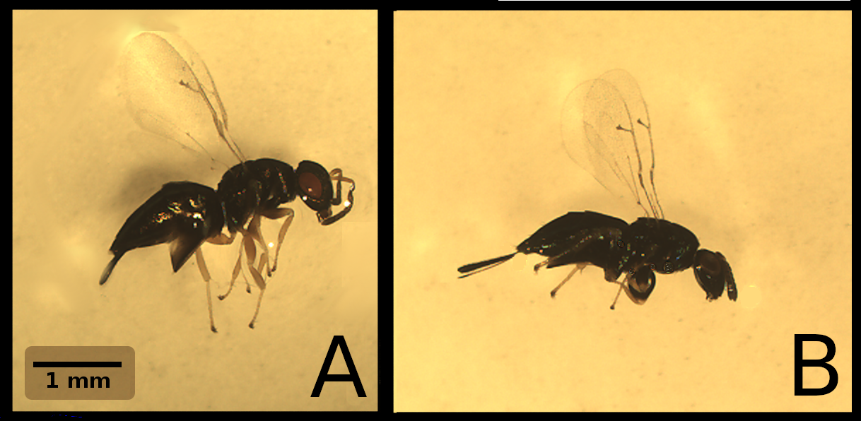
Figure 30.1: Fig wasps from two different species, (A) Het1 and (B) Het2. Wasps were collected from Baja, Mexico. Image modified from Duthie, Abbott, and Nason (2015).

Both fig wasp species in Figure 30.1 are unnamed. We can call the species in Figure 30.1A ‘Het1’ and the species in Figure 30.1B ‘Het2’. We might want to collect morphological measurements of fig wasp head, thorax, and abdomen lengths in these two species (Duthie et al., 2015). Table 30.1 shows these measurements for 11 wasps.

TABLE 30.1 Body segment length measurements (mm) from fig wasps of two species. Data were collected from Baja, Mexico.

Species	Head	Thorax	Abdomen
Het1	0.566	0.767	1.288
Het1	0.505	0.784	1.059
Het1	0.511	0.769	1.107
Het1	0.479	0.766	1.242
Het1	0.545	0.828	1.367
Het1	0.525	0.852	1.408
Het2	0.497	0.781	1.248
Het2	0.450	0.696	1.092
Het2	0.557	0.792	1.240
Het2	0.519	0.814	1.221
Het2	0.430	0.621	1.034

Intuitively, we might expect most of these measurements to be associated with one another. For example, if a fig wasp has a relatively long thorax, then it probably also has a relatively long abdomen (i.e., it could just be a big wasp). We can check this visually by plotting one variable on the x-axis and the other on the y-axis. Figure 30.2 does this for wasp thorax length (x-axis) and abdomen length (y-axis).

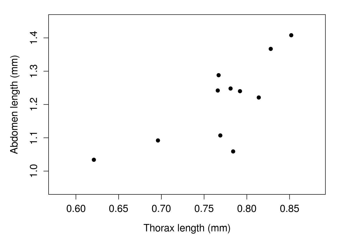
Figure 30.2: Example of a scatterplot in which fig wasp thorax length (x-axis) is plotted against fig wasp abdomen length (y-axis). Each point is a different fig wasp. Wasps were collected in 2010 in Baja, Mexico.

In Figure 30.2, each point is a different wasp from Table 30.1. For example, in the last row of Table 30.1, there is a wasp with a particularly low thorax length (0.621 mm) and abdomen length (1.034 mm). In the scatterplot, we can see this wasp represented by the point that is lowest and furthest to the left (Figure 30.2).

There is a clear association between thorax length and abdomen length in Figure 30.2. Fig wasps that have low thorax lengths also tend to have low abdomen lengths, and wasps that have high thorax lengths also tend to have high abdomen lengths. In this sense, the two variables are associated. More specifically, they are positively correlated. As thorax length increases, so does abdomen length.

30.2 Correlation coefficient

The correlation coefficient formalises the association described in the previous section. It gives us a single number that defines how two variables are correlated. We represent this number with the letter ‘\(r\)’, which can range from values of -1 to 1.⁷⁰ Positive values indicate that two variables are positively correlated, such that a higher value of one variable is associated with higher values of the other variable (as was the case with fig wasp thorax and abdomen measurements). Negative values indicate that two variables are negatively correlated, such that a higher values of one variable are associated with lower values of the other variable. Values of zero (or not significantly different from zero, more on this later) indicate that two variables are uncorrelated (i.e., independent of one another). Figure 30.3 shows scatterplots for four different correlation coefficients between values of \(x\) and \(y\).

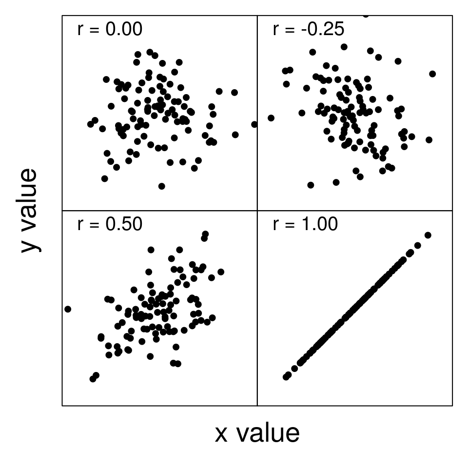
Figure 30.3: Examples of scatterplots with different correlation coefficients (r) between two variables (x and y).

We will look at two types of correlation coefficient, the Pearson product moment correlation coefficient and Spearman’s rank correlation coefficient. The two are basically the same; Spearman’s rank correlation coefficient is just a correlation of the ranks of values instead of the actual values.

30.2.1 Pearson product moment correlation coefficient

To understand the correlation coefficient, we need to first understand covariance. Section 12.3 introduced the variance (\(s^{2}\)) as a measure of spread in some variable \(x\),

\[s^{2} = \frac{1}{N - 1}\sum_{i = 1}^{N}\left(x_{i} - \bar{x} \right)^{2}.\]

The variance is actually just a special case of a covariance. The variance describes how a variable \(x\) covaries with itself. The covariance (\(cov_{x,y}\)) describes how a variable \(x\) covaries with another variable \(y\),

\[cov_{x, y} = \frac{1}{N - 1} \sum_{i = 1}^{N}\left(x_{i} - \bar{x} \right) \left(y_{i} - \bar{y} \right).\]

The \(\bar{x}\) and \(\bar{y}\) are the means of \(x\) and \(y\), respectively. Note that if \(x_{i} = y_{i}\), then the equation for \(cov_{x,y}\) is identical to the equation for \(s^{2}\) because \(\left(x_{i} - \bar{x} \right) \left(x_{i} - \bar{x} \right) = \left(x_{i} - \bar{x} \right)^{2}\).

What the equation for \(cov_{x,y}\) is describing is how variation in \(x\) relates to variation in \(y\). If a value of \(x_{i}\) is much higher than the mean \(\bar{x}\), and a value of \(y_{i}\) is much higher than the mean \(\bar{y}\), then the product of \(\left(x_{i} - \bar{x} \right)\) and \(\left(y_{i} - \bar{y} \right)\) will be especially high because we will be multiplying two large positive numbers together. If a value of \(x_{i}\) is much higher than the mean \(\bar{x}\), but the corresponding \(y_{i}\) is much lower than the mean \(\bar{y}\), then the product of \(\left(x_{i} - \bar{x} \right)\) and \(\left(y_{i} - \bar{y} \right)\) will be especially low because we will be multiplying a large positive number and a large negative number. Consequently, when \(x_{i}\) and \(y_{i}\) tend to deviate from their means \(\bar{x}\) and \(\bar{y}\) in a consistent way, we get either high or low values of \(cov_{x,y}\). If there is no such relationship between \(x\) and \(y\), then we will get \(cov_{x,y}\) values closer to zero.

The covariance can, at least in theory, be any real number. How low or high it is will depend on the magnitudes of \(x\) and \(y\), just like the variance. To get the Pearson product moment correlation coefficient⁷¹ (\(r\)), we need to standardise the covariance so that the minimum possible value of \(r\) is \(-1\) and the maximum possible value of \(r\) is 1. We can do this by dividing \(cov_{x,y}\) by the product of the standard deviation of \(x\) (\(s_{x}\)) and the standard deviation of \(y\) (\(s_{y}\)),

\[r = \frac{cov_{x,y}}{s_{x} \times s_{y}}.\]

This works because \(s_{x} \times s_{y}\) describes the total variation between the two variables, and the absolute value of \(cov_{x,y}\) cannot be larger than this total. We can again think about the special case in which \(x = y\). Since the covariance between \(x\) and itself is just the variance of \(x\) (\(s_{x}^{2}\)), and \(s_{x} \times s_{x} = s^{2}_{x}\), we end up with the same value on the top and bottom, and \(r = 1\) (i.e., \(x\) is completely correlated with itself).

We can expand \(cov_{x,y}\), \(s_{x}\), and \(s_{y}\) to see the details of the equation for \(r\),

\[r = \frac{\frac{1}{N - 1} \sum_{i = 1}^{N}\left(x_{i} - \bar{x} \right) \left(y_{i} - \bar{y} \right)}{\sqrt{\frac{1}{N - 1}\sum_{i = 1}^{N}\left(x_{i} - \bar{x} \right)^{2}} \sqrt{\frac{1}{N - 1}\sum_{i = 1}^{N}\left(y_{i} - \bar{y} \right)^{2}}}.\]

This looks like a lot, but we can clean the equation up a bit because the \(1 / (N-1)\) expressions cancel on the top and bottom of the equation,

\[r = \frac{\sum_{i = 1}^{N}\left(x_{i} - \bar{x} \right) \left(y_{i} - \bar{y} \right)}{\sqrt{\sum_{i = 1}^{N}\left(x_{i} - \bar{x} \right)^{2}} \sqrt{\sum_{i = 1}^{N}\left(y_{i} - \bar{y} \right)^{2}}}.\]

As with other statistics defined in this book, it is almost never necessary to calculate \(r\) by hand. Jamovi will make these calculations for us (The jamovi project, 2024). The reason for working through all of these equations is to help make the conceptual link between \(r\) and the variance of the variables of interest (Rodgers & Nicewander, 1988). To make this link a bit clearer, we can calculate the correlation coefficient of thorax and abdomen length from Table 30.1. We can set thorax to be the \(x\) variable and abdomen to be the \(y\) variable. Mean thorax length is \(\bar{x} = 0.770\), and mean abdomen length is \(\bar{y} = 1.210\). The standard deviation of thorax length is \(s_{x} = 0.06366161\), and the standard deviation of abdomen length is \(s_{y} = 0.1231806\). This gives us the numbers that we need to calculate the bottom of the fraction for \(r\), which is \(s_{x} \times s_{y} = 0.007841875\). We now need to calculate the covariance on the top. To get the covariance, we first need to calculate \(\left(x_{i} - \bar{x} \right) \left(y_{i} - \bar{y} \right)\) for each row (\(i\)) in Table 30.1. For example, for row 1, \(\left(0.767 - 0.770\right) \left(1.288 - 1.210\right) = -0.000234.\) For row 2, \(\left(0.784 - 0.770\right) \left(1.059 - 1.210\right) = -0.002114.\) We continue this for all rows. Table 30.2 shows the thorax length (\(x_{i}\)), abdomen length (\(y_{i}\)), and \(\left(x_{i} - \bar{x} \right) \left(y_{i} - \bar{y} \right)\) for rows \(i = 1\) to \(i = 11\).

TABLE 30.2 Measurements of 11 fig wasp thorax and abdomen lengths (mm). The fourth column shows the product of the deviations of each measurement from the mean, where mean thorax length is 0.770 and mean abdomen length is 1.210.

Row (i)	Thorax	Abdomen	Squared Deviation
1	0.767	1.288	-0.000234
2	0.784	1.059	-0.002114
3	0.769	1.107	0.000103
4	0.766	1.242	-0.000128
5	0.828	1.367	0.009106
6	0.852	1.408	0.01624
7	0.781	1.248	0.000418
8	0.696	1.092	0.008732
9	0.792	1.240	0.00066
10	0.814	1.221	0.000484
11	0.621	1.034	0.02622

If we sum up all of the values in the column ‘Squared Deviation’ from Table 30.2, we get a value of 0.059487. We can multiply this value by \(1 / (N - 1)\) to get the top of the equation for \(r\) (i.e., \(cov_{x,y}\)), \((1 / (11-1)) \times 0.059487 = 0.0059487\). We now have all of the values we need to calculate \(r\) between fig wasp thorax and abdomen length,

\[r_{x,y} = \frac{0.0059487}{0.06366161 \times 0.1231806}.\]

Our final value is \(r_{x, y} = 0.759\). As suggested by the scatterplot in Figure 30.2, thorax and abdomen lengths are highly correlated. We will test whether or not this value of \(r\) is statistically significant in Section 30.3, but first we will introduce the Spearman’s rank correlation coefficient.

30.2.2 Spearman’s rank correlation coefficient

We have seen how the ranks of data can be substituted in place of the actual values. This has been useful when data violate the assumptions of a statistical test, and we need a non-parametric test instead (e.g., Wilcoxon signed rank test, Mann-Whitney U test, or Kruskal-Wallis H test). We can use the same trick for the correlation coefficient. Spearman’s rank correlation coefficient is calculated the exact same way as the Pearson product moment correlation coefficient, except on the ranks of values. To calculate Spearman’s rank correlation coefficient for the fig wasp example in the previous section, we just need to rank the thorax and abdomen lengths from 1 to 11, then calculate \(r\) using the rank values instead of the actual measurements of length. Table 30.3 shows the same 11 fig wasp measurements as Tables 30.1 and 30.2, but with columns added to show the ranks of thorax and abdomen lengths.

TABLE 30.3 Measurements of 11 fig wasp thorax and abdomen lengths (mm) and their ranks.

Wasp (i)	Thorax	Thorax Rank	Abdomen	Abdomen Rank
1	0.767	4	1.288	9
2	0.784	7	1.059	2
3	0.769	5	1.107	4
4	0.766	3	1.242	7
5	0.828	10	1.367	10
6	0.852	11	1.408	11
7	0.781	6	1.248	8
8	0.696	2	1.092	3
9	0.792	8	1.240	6
10	0.814	9	1.221	5
11	0.621	1	1.034	1

Note from Table 30.3 that the lowest value of Thorax is 0.621, so it gets a rank of 1. The highest value of Thorax is 0.852, so it gets a rank of 11. We do the same for abdomen ranks. To get Spearman’s rank correlation coefficient, we just calculate \(r\) using the ranks. The ranks number from 1 to 11 for both variables, so the mean rank is 6 and the standard deviation is 3.317 for both thorax and abdomen ranks. We can then go through each row and calculate \(\left(x_{i} - \bar{x} \right) \times \left(y_{i} - \bar{y} \right)\) using the ranks. For the first row, this gives us \(\left(4 - 6 \right) \left(9 - 6 \right) = -6\). If we do this same calculation for each row and sum them up, then multiply by \(1/(N-1)\), we get a value of 6.4. To calculate \(r\),

\[r_{\mathrm{rank}(x),\mathrm{rank}(y)} = \frac{6.4}{3.317 \times 3.317}\]

Our Spearman’s rank correlation coefficient is therefore \(r = 0.582\), which is a bit lower than our Pearson product moment correlation was. The key point here is that the definition of the correlation coefficient has not changed; we are just using the ranks of our measurements instead of the measurements themselves. The reason why we might want to use Spearman’s rank correlation coefficient instead of the Pearson product moment correlation coefficient is explained in the next section.

30.3 Correlation hypothesis testing

We often want to test if two variables are correlated. In other words, is \(r\) significantly different from zero? We therefore want to test the null hypothesis that \(r\) is not significantly different from zero.

• \(H_{0}:\) The population correlation coefficient is zero.
• \(H_{A}:\) The correlation coefficient is significantly different from zero.

Note that \(H_{A}\) above is for a two-tailed test, in which we do not care about direction. We could also use a one-tailed test if our \(H_{A}\) is that the correlation coefficient is greater than (or less than) zero.

How do we actually test the null hypothesis? As it turns out, the sample correlation coefficient (\(r\)) will be approximately t-distributed around a true correlation (\(\rho\)) with a t-score defined by \(r - \rho\) divided by its standard error (\(\mathrm{SE}(r)\))⁷²,

\[t = \frac{r - \rho}{\mathrm{SE}(r)}.\]

Since our null hypothesis is that variables are uncorrelated, \(\rho = 0\). Jamovi will use this equation to test whether or not the correlation coefficient is significantly different from zero (The jamovi project, 2024). The reason for presenting it here is to show the conceptual link to other hypothesis tests in earlier chapters. In Section 22.1, we saw that the one sample t-test defined \(t\) as the deviation of the sample mean from the true mean, divided by the standard error. Here we are doing the same for the correlation coefficient. One consequence of this is that, like the one sample t-test, the test of the correlation coefficient assumes that \(r\) will be normally distributed around the true correlation \(\rho\). If this is not the case, and the assumption of normality is violated, then the test might have a misleading Type I error rate.

To be cautious, we should check whether or not the variables that we are correlating are normally distributed (especially if the sample size is small). If they are normally distributed, then we can use the Pearson’s product moment correlation to test the null hypothesis. If the assumption of normality is violated, then we might consider using the non-parametric Spearman’s rank correlation coefficient instead. The fig wasp thorax and abdomen lengths from Table 30.1 are normally distributed, so we can use the Pearson product moment correlation coefficient to test whether or not the correlation between these two variables is significant. In jamovi, the t-score is not even reported as output when using a correlation test. We only see \(r\) and the p-value (Figure 30.4).

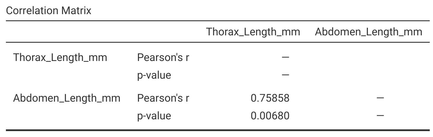
Figure 30.4: Jamovi output for a test of the null hypothesis that thorax length and abdomen length are not significantly correlated in a sample of fig wasps collected in 2010 from Baja, Mexico.

From Figure 30.4, we can see that the sample \(r = 0.75858\), and the p-value is \(P = 0.00680\). Since our p-value is less than 0.05, we can reject the null hypothesis that fig wasp thorax and abdomen lengths are not correlated (an interactive application⁷³ can make this more intuitive).

References

Duthie, A. B., Abbott, K. C., & Nason, J. D. (2015). Trade-offs and coexistence in fluctuating environments: evidence for a key dispersal-fecundity trade-off in five nonpollinating fig wasps. American Naturalist, 186(1), 151–158. https://doi.org/10.1086/681621

Rahman, N. A. (1968). A Course in Theoretical Statistics (p. 542). Charles Griffin & Company, London.

Rodgers, J. L., & Nicewander, W. (1988). Thirteen ways to look at the correlation coefficient. American Statistician, 42(1), 59–66.

The jamovi project. (2024). Jamovi (version 2.5). https://www.jamovi.org

---

70. Note that \(r\) is the sample correlation coefficient, which is an estimate of the population correlation coefficient. The population correlation coefficient is represented by the Greek letter ‘\(\rho\)’ (‘rho’), and sometimes the sample correlation coefficient is represented as \(\hat{\rho}\).↩︎

71. We can usually just call this the ‘correlation coefficient’.↩︎

72. We can calculate the standard error of \(r\) as (Rahman, 1968), \[\mathrm{SE}(r) = \sqrt{\frac{1 - r^{2}}{N - 2}}.\] But this is not necessary to ever do by hand. Note that we lose two degrees of freedom (\(N - 2\)), one for calculating each variable mean.↩︎

73. https://bradduthie.github.io/stats/app/corr_click/↩︎