Chapter 34 Practical. Using regression
This chapter focuses on practical exercises to apply the concepts in Chapter 32 and Chapter 33 in jamovi (The jamovi project, 2024). The five exercises in this practical will apply simple linear regression (Exercises 34.1, 34.2, and 34.5) or multiple regression (34.3 and 34.4). The dataset used in this practical is inspired by the work of Dr Carmen Carmona, Dr François-Xavier Joly, and Prof Jens-Arne Subke80. Their work focuses on carbon storage in Gabon.
When biomass is burned, a large proportion of its stored carbon is emitted into the atmosphere in the form of carbon dioxide, but some of it remains sequestered in the soil due to incomplete combustion (Santín et al., 2016). This pyrogenic organic carbon can persist in the soil for long periods of time and has positive effects on soil properties (Reisser et al., 2016). In this chapter, we will look at how environmental data might be used to test what factors affect the concentration of pyrogenic carbon in the soil. We will use the fire carbon dataset81. This dataset includes variables for soil depth (cm), fire frequency (total number of years in which a fire occurred during the past 20 years), mean yearly temperature (degrees Celsius), mean monthly rainfall (millimetres per squared metre per year, \(\mathrm{mm\:m^{-2}\:yr^{-1}}\)), total soil organic carbon (SOC, as percentage of soil by weight), pyrogenic carbon (PyC, as percentage of soil organic carbon by weight), and soil pH.
34.1 Predicting pyrogenic carbon from soil depth
In this first activity, we will fit a linear regression to predict pyrogenic carbon (PyC) from soil depth (depth). Before doing this, what is the independent variable, and what is the dependent variable?
Independent variable: __________________
Dependent variable: ___________________
What is the sample size of this dataset?
\(N =\) ________________
Before running any statistical test, it is always a good idea to plot the data. Recall from Section 31.4 how to build a scatterplot in jamovi. Navigate to the ‘Exploration’ button from the jamovi toolbar, then choose the ‘Scatterplot’ option from the pull-down menu. Place the independent variable that you identified above on the x-axis, and place the dependent variable on the y-axis. To get the line of best fit, choose ‘Linear’ under the options below under Regression line. Describe the scatterplot that is produced in the jamovi panel to the right.
Recall the four assumptions of linear regression from Section 32.6. We will now check three of these assumptions (we will just have to trust that depth has been measured accurately in the field because there is no way to check). There are two assumptions that we can check using the scatterplot. The first assumption is that the relationship between the independent and dependent variable is linear. Is there any reason to be suspicious of this assumption? In other words, does the scatterplot show any evidence of a curvilinear pattern in the data?
The second assumption that we can check with the scatterplot is the assumption of homoscedasticity. In other words, does the variance change along the range of the independent variable (i.e., x-axis)?
Assuming that these two assumptions are not violated, we can now check the last assumption that the residual values are normally distributed around the regression line. To do this, we need to build the linear regression. From the ‘Analyses’ tab of jamovi, select the ‘Regression’ button, then choose ‘Linear regression’ from the pull-down menu. A new panel called ‘Linear regression’ will open. The dependent variable ‘PyC’ should go in the ‘Dependent Variable’ box to the right. The independent variable ‘depth’ should go in the ‘Covariates’ box (Figure 34.1).
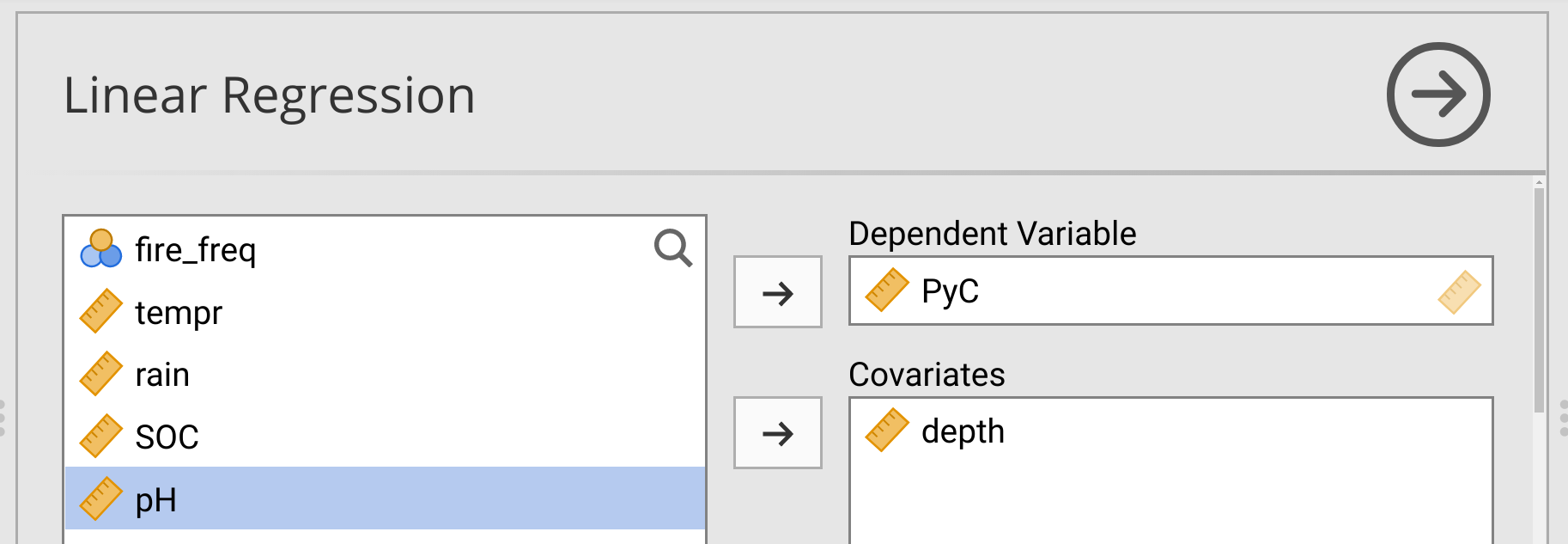
Figure 34.1: Jamovi interface for running a linear regression model to predict pyrogenic carbon (PyC) from soil depth (depth).
We can check the assumption that the residuals are normally distributed in multiple ways. To do this, find the pull-down menu called ‘Assumption Checks’ in the left panel of jamovi, and check boxes for ‘Normality test’, ‘Q-Q plot of residuals’, and ‘Residual plots’. Output will appear in the jamovi panel to the right. The first assumption check will be a table providing the results of a Shapiro-Wilk test of normality on the residuals (see Section 32.2) of the linear regression model. In your own words, what is this test doing? Drawing a picture might help to explain.
What is the p-value of the Shapiro-Wilk test of normality?
\(P =\) __________________
Based on the above p-value, is it safe to conclude that the residuals are normally distributed?
Conclusion: _____________________
The assumption checks output also includes a Q-Q plot. Below the Q-Q plot, there is a residual plot that shows ‘Fitted’ on the x-axis and ‘Residuals’ on the y-axis. What this tells us is the relationship between the PyC values that are predicted by the regression equation (x-axis, i.e., what our equation predicts PyC will be for a particular depth) and the actual PyC values in the data (y-axis). Visually, this is the equivalent of taking the line of best fit from the first scatterplot that you made and moving it (and the points around it) so that it is horizontal at y = 0. It is good to try to take a few moments to understand this because it will help reinforce the concept of residual values, but in practice we can base our conclusion about residual normality on the Shapiro-Wilk test as done above.
Having checked all of the assumptions of a linear regression model, we can finally test whether or not our model is statistically significant. Find the pull-down called ‘Model Fit’ underneath the linear regression panel, then make sure that the boxes for \(R^{2}\) and ‘F test’ are checked. A new table will open up in the right panel called ‘Model Fit Measures’. Write the output statistics from this table below:
\(R^{2} =\) ________________
\(F =\) ________________
\(df1 =\) _______________
\(df2 =\) _______________
\(P =\) ______________
Based on these statistics, what percentage of the variation in pyrogenic carbon is explained by the linear regression model?
What null hypothesis does the p-value above test? (hint, see Section 32.7.1)
\(H_{0}\): __________________
Do we reject or fail to reject \(H_{0}\)?
Lastly, have a look at the output table called ‘Model Coefficients - PyC’. This is the same kind of table that was introduced in Section 32.7.4. From this table, what are the coefficient estimates for the intercept and slope (i.e., depth)?
Intercept: _______________
Slope: ________________
Find the p-values associated with the intercept and slope. What null hypotheses are we testing when inspecting these p-values? (hint, see Section 32.7.2 and Section 32.7.3)
Intercept \(H_{0}\): _____________
Slope \(H_{0}\): _____________
Finally, what can we conclude about the relationship between depth and pyrogenic carbon storage?
34.2 Predicting pyrogenic carbon from fire frequency
Now, we can try to predict pyrogenic carbon (PyC) from fire frequency (fire_freq). This exercise will be a bit more self-guided than the previous exercise. To begin, make a scatterplot with fire frequency on the x-axis and PyC on the y-axis. Add a linear regression line, then paste the plot or sketch it below (if sketching, no need for too much detail, just the trend line and 10–15 points is fine).
Next, check the linear regression assumptions of linearity, normality, and homoscedasticity, as we did in the previous exercise. Do all these assumptions appear to be met?
Linearity: ______________
Normality: _____________
Homoscedasticity: ______________
Next, run the linear regression model. To check for the assumption of normality, you should have already specified a regression model with fire frequency as the independent variable and PyC as the dependent variable. Using the same protocol as the previous exercise, what percentage of the variation in PyC is explained by the regression model?
Variation explained: _________________
Is the overall model statistically significant? How do you know?
Model significance: ____________________
Are the intercept and slope significantly different from zero?
Intercept: ______________
Slope: ____________
Write the intercept (\(b_{0}\)) and slope (\(b_{1}\)) of the regression below.
\(b_{0} =\) ____________
\(b_{1} =\) ____________
Using these values for the intercept and the slope, write the regression equation to predict pyrogenic carbon (PyC) from fire frequency (fire_freq).
Using this equation, what would be the predicted PyC for a location that had experienced 10 fires in the past 20 years (i.e., fire_freq = 10)?
One final note for this exercise. In the Linear Regression panel of jamovi, scroll all the way down to the last pull-down menu called ‘Save’. Check the boxes for ‘Predicted values’ and ‘Residuals’. When you return to the ‘Data’ tab in jamovi, you will see two new columns of data that jamovi has inserted. One column will be the predicted values for the model, i.e., the value that the model predicts for PyC given the fire frequency in the observation (i.e., row). The other column will be the residual value of each observation. Explain what these two columns of data represent in terms of the scatterplot you made at the start of this exercise. In other words, where would the predicted and residual values be located on the scatterplot?
34.3 Multiple regression depth and fire frequency
In this exercise, we will run a multiple regression to predict pyrogenic carbon (PyC) from fire frequency (fire_freq) and depth. Write down what the independent and dependent variable(s) are for this regression.
Independent: ___________________
Dependent: _________________
To begin the multiple regression, select the ‘Regression’ button in the Analysis tab of jamovi, then choose ‘Linear regression’ as you did in the first two exercises. Place the dependent variable in the ‘Dependent Variable’ box and both independent variables in the ‘Covariates’ box. As with the previous exercise, check the linear regression assumptions of linearity, normality, and homoscedasticity. Do all these assumptions appear to be met?
Linearity: ______________
Normality: _____________
Homoscedasticity: ______________
Make sure to select \(R^{2}\), Adjusted \(R^{2}\), and F test under the Model Fit options. Report these values from the Model Fit Measures output table below.
\(R^{2} =\) ________________________
Adjusted \(R^{2} =\) ___________________
\(F =\) _________________
\(P =\) _________________
Explain why the Adjusted \(R^{2}\) is less than the \(R^{2}\) value. Which one is most appropriate to use for interpreting the multiple regression?
What is the null hypothesis tested with the \(F\) value and the p-value shown in the Model Fit Measures table?
\(H_{0}\): ____________________
Based on the Overall Model Test output, should you reject or not reject \(H_{0}\)?
Next, have a look at the Model Coefficients - PyC table. What can you conclude about the significance of the Intercept, and the partial regression coefficients for fire frequency and depth?
Using the partial regression coefficient estimates, fill in the equation below,
\[PyC = (\:\:\:\:\:\:\:\:\:\:\:\:\:\:) + (\:\:\:\:\:\:\:\:\:\:\:\:\:\:)fire\_freq + (\:\:\:\:\:\:\:\:\:\:\:\:\:\:)depth.\]
Next, use this to predict the PyC for a fire frequency of 12 and a depth of 60 cm.
PyC = __________________
Contrast soil depth as a predictor of PyC in this multiple regression model versus the simple linear regression model in the first exercise. Has the significance of soil depth as an independent variable changed? Based on what you know about the difference between simple linear regression and multiple regression, why might this be the case?
34.4 Large multiple regression
Suppose that as scientists, we hypothesise that soil depth, fire frequency, and soil pH will all affect pyrogenic carbon storage. Run a multiple regression model with soil depth, fire frequency, and soil pH all as independent variables and pyrogenic carbon as a dependent variable. Fill in the Model Coefficients output in Table 34.1.
| Estimate | Std. Error | t Value | Pr(>|t|) | |
|---|---|---|---|---|
| (Intercept) | 0.34591 | 2.85888 | ||
| depth | 8e-04 | -0.07411 | ||
| fire_freq | 0.00394 | 14.42303 | ||
| pH | 0.05679 | -0.27886 |
From the Model Fit Measures table, what is the \(R^{2}\) and Adjusted \(R^{2}\) of this model?
\(R^{2}\): _______________
Adjusted \(R^{2}\): ______________
Compare these values to the \(R^{2}\) and Adjusted \(R^{2}\) from the multiple regression in the previous exercise (i.e., the one without pH as an independent variable). Is the \(R^{2}\) value of this model higher or lower than the multiple regression model without pH?
Is the Adjusted \(R^{2}\) value of this model higher or lower than the multiple regression model without pH?
Based on what you know from Section 33.1, explain why the \(R^{2}\) and Adjusted \(R^{2}\) might have changed in different directions with the addition of a new independent variable.
Finally, use the equation of this new model to predict PyC for a soil sample at a depth of 0, fire frequency of 0, and pH of 6.
34.5 Predicting temperature from fire frequency
In this last brief exercise, suppose that we wanted to predict temperature (tempr) from fire frequency (fire_freq). Run some checks of the assumptions underlying linear regression (see Section 32.6). What assumption(s) appear as though they might be violated for this simple regression? Explain how you figured this out.
References
Please note that the data in this practical are for educational purposes only. They are not the data that were actually collected by the researchers.↩︎