Chapter 25 Multiple comparisons
In the Section 24.2 ANOVA example, we rejected the null hypothesis that all fig wasp species have the same mean wing length. We can therefore conclude that at least one species has a different mean wing length than the rest; can we determine which one(s)? We can try to find this out using a post hoc comparison (post hoc is Latin for ‘after the event’). That is, after we have rejected the null hypothesis in the one-way ANOVA, we can start comparing individual groups (Het1 vs Het2, Het1 vs LO1, etc.). Nevertheless, we need some way to correct for the Type I error problem explained at the beginning of Chapter 24. That is, if we run a large enough number of t-tests, then we are almost guaranteed that we will find a significant difference between means (\(P < 0.05\)) where none really exists. A way to avoid this inflated Type I error rate is to set our significance threshold to be lower than the usual \(\alpha = 0.05\). We can, for example, divide our \(\alpha\) value by the total number of pair-wise t-tests that we run. This is called a Bonferroni correction (Dytham, 2011), and it is an especially cautious approach to post hoc comparisons between groups (Narum, 2006). For the fig wasp wing lengths, recall that there are 10 possible pairwise comparisons between the five species. This means that if we were to apply a Bonferroni correction and run 10 separate t-tests, then we would only conclude that species mean wing lengths were different when \(P < 0.005\) instead of \(P < 0.05\).
Another approach to correcting for multiple comparisons is a Tukey’s honestly significant difference test (Tukey’s HSD, or just a ‘Tukey test’). The general idea of a Tukey test is the same as the Bonferroni. Multiple t-tests are run in a way that controls the Type I error rate so that the probability of making a Type I error across the whole set of comparisons is fixed (e.g., at \(\alpha = 0.05\)). The Tukey test does this by using a modified t-test, with a t-distribution called the ‘studentised range distribution’ that applies the range of mean group values (i.e., \(\max(\bar{x}) - \min(\bar{x})\)) and uses the sample variance across the groups with the highest and lowest sample means (Box et al., 1978; Tukey, 1949).
Multiple comparisons tests can be run automatically in jamovi. Figure 25.1 shows a post hoc comparisons table for all pair-wise combinations of fig wasp species wing length means.
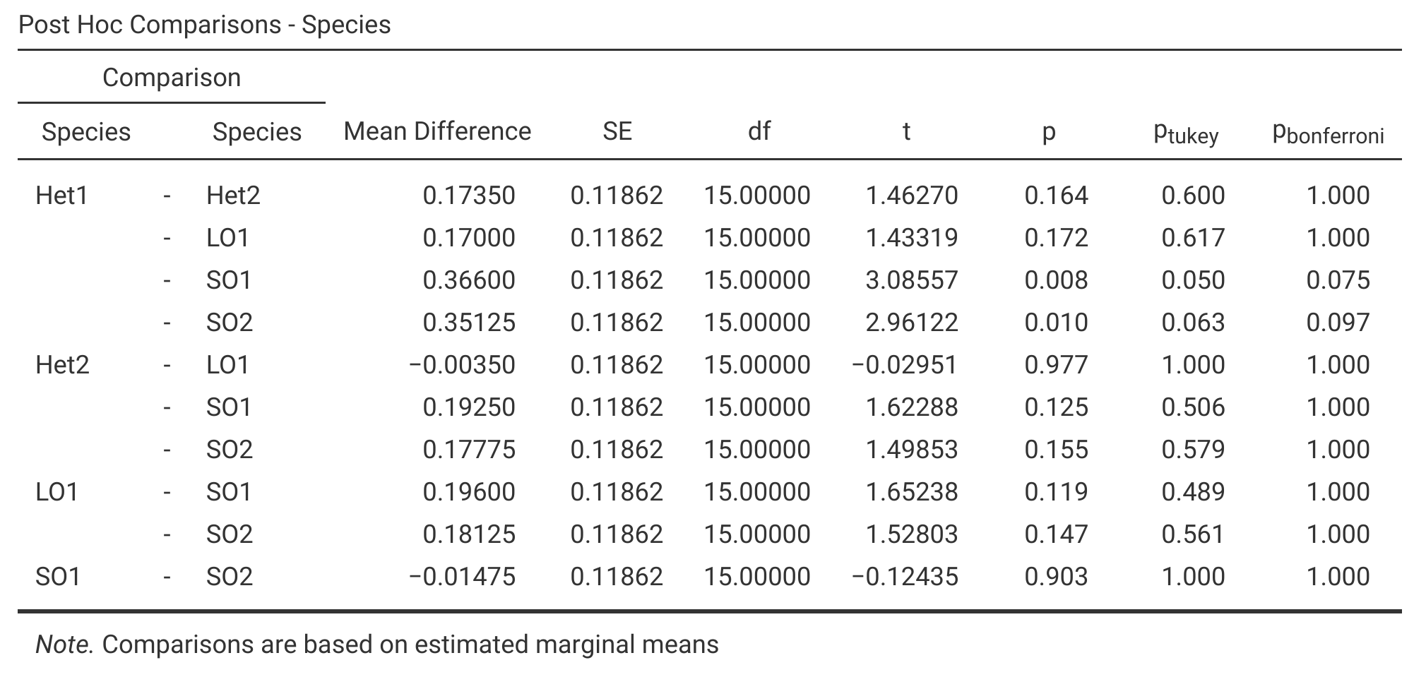
Figure 25.1: Jamovi output showing a table of 10 post hoc comparisons between species mean wing lengths for five different species of fig wasps. The last three columns show the uncorrected p-value (p), a p-value obtained from a Tukey test, and a p-value obtained from a Bonferroni correction. Species wing length measurements were collected in 2010 near La Paz in Baja, Mexico.
The column ‘p’ in Figure 25.1 is the uncorrected p-value, i.e., the p-value that a t-test would produce without any correction for multiple comparisons. The columns \(p_{\mathrm{tukey}}\) and \(p_{\mathrm{bonferroni}}\) show corrected p-values for the Tukey test and Bonferroni corrected t-test, respectively. We can interpret these p-values as usual, concluding that two species have different means if \(P < 0.05\) (i.e., jamovi does the correction for us; we do not need to divide \(\alpha = 0.05\) to figure out what the significance threshold should be, given the Bonferroni correction).
Note that from Figure 25.1, it appears that both the Tukey test and the Bonferroni correction fail to find that any pair of species have significantly different means. This does not mean that we have done the test incorrectly. The multiple comparisons tests are asking a slightly different question than the one-way ANOVA. The multiple comparisons tests are testing the null hypothesis that two particular species have the same mean wing lengths. The one-way ANOVA tested the null hypothesis that all species have the same mean, and our result for the ANOVA was barely below the \(\alpha = 0.05\) threshold (\(P = 0.042\)). The ANOVA also has more statistical power because it makes use of all 20 measurements in the dataset, not just a subset of measurements between two of the five species. It is therefore not particularly surprising or concerning that we rejected \(H_{0}\) for the ANOVA, but the multiple comparisons tests failed to find any significant difference between group means.