Chapter 28 Practical. ANOVA and associated tests
This chapter focuses on applying the concepts from Chapters 24-27 in jamovi (The jamovi project, 2024). The focus will be on ANOVA and associated tests, with five exercises in total. The data for this chapter are inspired by the work of Dr Lidia de Sousa Teixeira at the University of Stirling (de Sousa Teixeira, 2022). This doctoral work included a nutrient analysis of agricultural soil in different regions of Angola. Measuring soil nutrient concentrations is essential for assessing soil quality, and these data include measurements of Nitrogen (N), Phosphorus (P), and Potassium (K) concentrations. Here we will focus on testing whether or not the concentrations of N, P, and K differ among two different sites and three soil profiles (upper, middle, and lower). This chapter uses the Angola soils dataset63. All concentrations of Nitrogen, Phosphorus, and Potassium are given in parts per million (ppm).
28.1 One-way ANOVA (site)
Suppose that we first want to test whether or not mean Nitrogen concentration is the same in different sites. Notice that there are only two sites in the dataset: Funda and Bailundo. We could therefore also use an Independent samples t-test. We will do this first, then compare the t-test output to the ANOVA output. What are the null (\(H_{0}\)) and alternative (\(H_{A}\)) hypotheses for the t-test?
\(H_{0}:\) ____________________
\(H_{A}:\) ____________________
Before running a t-test, remember that we need to check the assumptions of a t-test to see if any of them are violated (see Section 22.4). Use the Assumption Checks in jamovi as we did in Section 23.4 to test for normality and homogeneity of variances in Nitrogen concentration. What can you conclude from these two tests?
Normality conclusion: ___________________________
Homogeneity of variances conclusion: ______________
Given the conclusions from the checks of normality and homogeneity of variances above, what kind of test should you use to see if the mean Nitrogen concentration is significantly different in Funda versus Bailundo?
Test: __________________
Run the test above in jamovi. What is the p-value of the test, and what conclusion do you make about Nitrogen concentration at the two sites?
\(P =\) _________________
Conclusion: ____________________
Now we will use an ANOVA to test if the mean Nitrogen concentration differs between sites. Remember from Chapter 24 that the ANOVA compares the variance among groups to the variance within groups, calculating an F-statistic and finding where it is in the null F-distribution. To run an ANOVA, navigate to the ‘Analyses’ tab in jamovi, then select the ‘ANOVA’ button in the toolbar. From the ANOVA pull-down, select ‘One-Way ANOVA’. After selecting the one-way ANOVA, a familiar interface will open up. Place ‘Nitrogen’ in the Dependent Variables box and ‘Site’ in the Grouping Variable box. Although we have already checked the assumptions of normality and homogeneity of variances when we ran the t-test, check these boxes under Assumption Checks too (Figure 28.1).
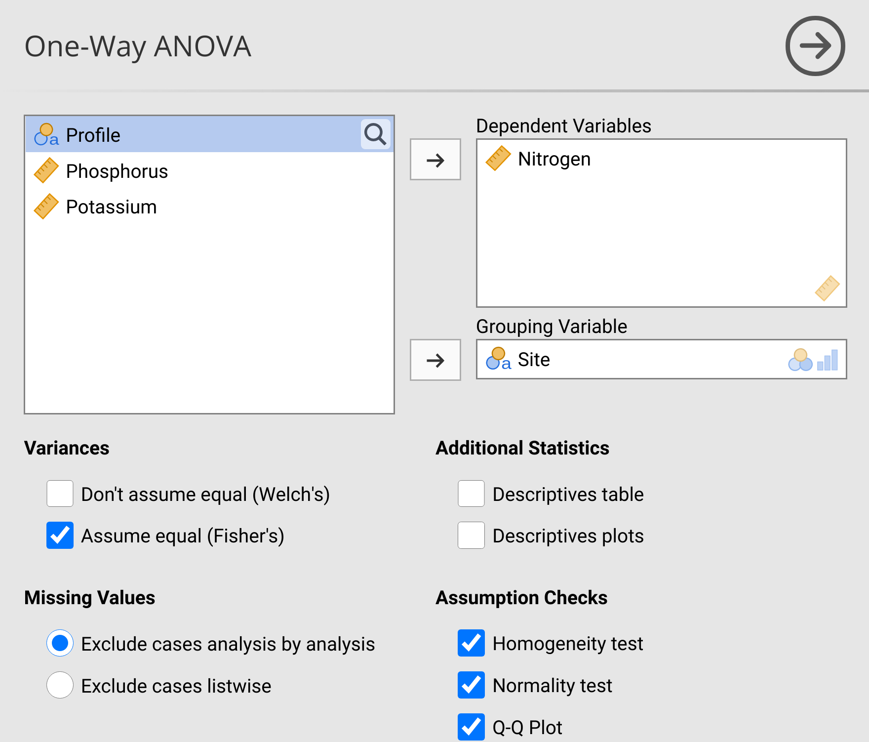
Figure 28.1: Jamovi interface for running a one-way ANOVA to test if Nitrogen concentration (ppm) differs among sites in the soils of Angola. Data for this test were inspired by the doctoral thesis of Dr Lidia de Sousa Teixeira.
Confirm that the Shapiro-Wilk test of normality and Levene’s test of homogeneity of variances are consistent with what you concluded when testing the assumptions of the t-test above. Since there is no reason to reject the null hypothesis that group variances are equal, we can use Fisher’s One-Way ANOVA by checking ‘Assume equal (Fisher’s)’ under Variances. A table called ‘One-Way ANOVA’ will appear in the panel on the right. Write down the test statistic (\(F\)), degrees of freedom, and p-value from this table below.
\(F =\) _______________
\(df1 =\) _______________
\(df2 =\) _______________
\(P =\) _______________
Remember from Chapter 24 that the ANOVA calculates an F-statistic (mean variance among groups divided by mean variance withing groups). This F-statistic is then compared to the null F-distribution with the correct degrees of freedom to calculate the p-value. You can use the interactive app to visualise this from the above jamovi output64. To do this, move the ‘Variance 1’ slider in the app until it is approximately equal to \(F\), then change \(df1\) and \(df2\) to the values above. From the interactive app, what is the approximate area under the curve (i.e., orange area) where the \(F\) value on the x-axis is greater than your calculated \(F\)?
\(P =\) _________________
Slide the ‘Variance 1’ to the left now until you find the \(F\) value where the probability density in the tail (orange) is about \(P = 0.05\). Approximately, what is this threshold \(F\) value above which we will reject the null hypothesis?
Approximate threshold \(F\): __________________
What should you conclude regarding the null hypothesis that sites have the same mean?
Conclusion: _________________
Look again at the p-value from the one-way ANOVA output and the Student’s t-test output. Are the two values the same, or different? Why might this be?
Next, we will run a one-way ANOVA to test the null hypothesis that all profiles have the same mean Nitrogen concentration.
28.2 One-way ANOVA (profile)
We will now run an ANOVA to see if Nitrogen concentration differs among profiles. In this dataset, there are lower, middle, and upper profiles, which refer to the location along a slope from which soil samples were obtained. Using the same approach as the previous Exercise 28.1, we will run a one-way ANOVA with profile as the independent variable instead of site. Again, navigate to the ‘Analyses’ tab in jamovi, then select the ‘ANOVA’ button in the toolbar. From the ANOVA pull-down menu, select ‘One-Way ANOVA’. First check the assumptions of normality and homogeneity of variances. What can you conclude?
Normality conclusion: ___________________________
Homogeneity of variances conclusion: ______________
It appears that the assumptions of normality and homogeneity of variances are met. We can therefore proceed with the one-way ANOVA. Run the one-way ANOVA with the assumption of equal variances (i.e., Fisher’s test). What are the output statistics in the One-Way ANOVA table?
\(F =\) _______________
\(df1 =\) _______________
\(df2 =\) _______________
\(P =\) _______________
From these statistics, what do you conclude about the difference in Nitrogen concentration among profiles?
Conclusion: _____________________
In the previous Exercise 28.1, we used an interactive app to visualise the relationship between the F-statistic and the p-value. We can do the same thing with the distrACTION module in jamovi. To do this, go to the distrACTION option in the jamovi toolbar and select ‘F-Distribution’ from the pull-down menu. Place the \(df1\) and \(df2\) from the One-Way ANOVA table into the df1 and df2 boxes under Parameters (ignore \(\lambda\)). Under Function, select ‘Compute probability’, then place the \(F\) value from the One-Way ANOVA table in the box for x1. We want the upper tail of the \(F\) probability distribution, so choose \(P(X \geq x1)\) from the radio buttons below. Write down the ‘Probability’ value from the Results table in the panel to the right.
Probability: _________________
Note that this is the same value (perhaps with a rounding error) as the p-value from the One-Way ANOVA table above. We can also find the threshold value of \(F\), above which we will reject the null hypothesis. To do this, check the ‘Compute quantile’ box and set p = 0.95 in the box below. From the Results table, what is the critical \(F\) value (‘Quantile’), above which we would reject the null hypothesis that all groups have the same mean?
Critical \(F\) value: ________________
Note that the objective of working this out in the distrACTION module (and with the interactive app) is to help explain what these different values in the One-Way ANOVA table actually mean. To actually test the null hypothesis, the One-Way ANOVA output table is all that we really need.
Finally, note that in the ANOVA pull-down menu from the jamovi toolbar, the option ‘ANOVA’ is just below the ‘One-way ANOVA’ that we used in this exercise and Exercise 28.1. This is just a more general tool for running an ANOVA, which includes the two-way ANOVA that we will use in Exercise 28.5 below. For now, give this a try by selecting ‘ANOVA’ from the pull-down menu. In the ANOVA interface, place ‘Nitrogen’ into the ‘Dependent Variable’ box and ‘Profile’ in the ‘Fixed Factors’ box (Figure 28.2).
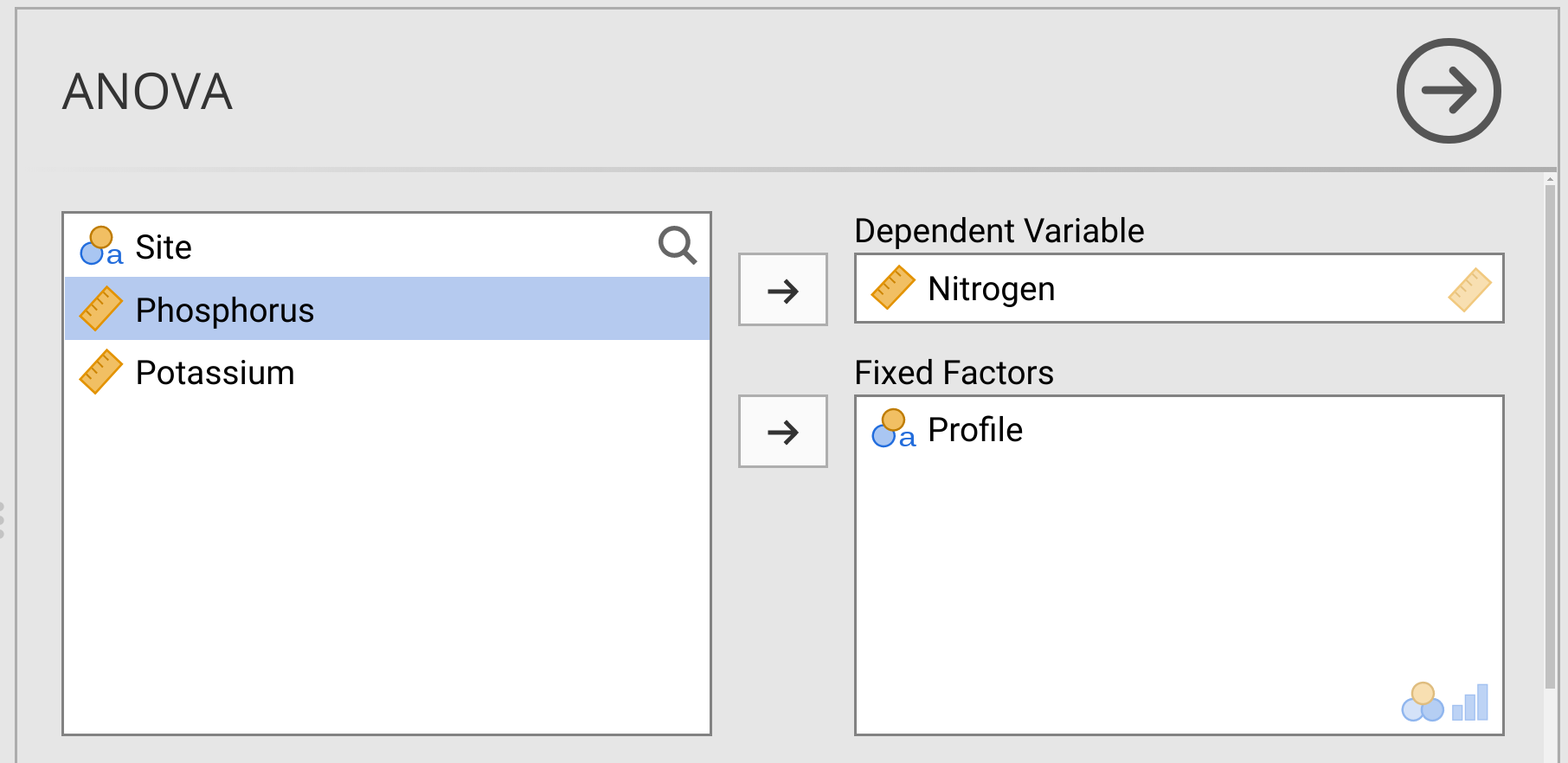
Figure 28.2: Jamovi interface for running an ANOVA to test if Nitrogen concentration (ppm) differs among soil profiles in Angola. Data for this test were inspired by the doctoral thesis of Dr Lidia de Sousa Teixeira.
The output in the right panel shows an ANOVA table. It includes the sum of squares of the among-group (Profile) and within-group (Residuals) sum of squares and mean square. This is often how ANOVA results are presented in the literature. Fill in the table below (Table 28.1) with the information for degrees of freedom, \(F\), and \(p\).
| Sum of Squares | df | Mean Square | F | p | |
|---|---|---|---|---|---|
| Profile | 16888.18606 | 8444.09303 | |||
| Residuals | 118092.02927 | 2460.25061 |
Now that we have established from the one-way ANOVA that mean Nitrogen concentration is not the same across all soil profiles, we can use a test of multiple comparisons to test which profile(s) are significantly different from one another.
28.3 Multiple comparisons
In this exercise, we will pick up where we left off in the ANOVA of Exercise 28.2. We have established that not all soil profiles have the same mean. Next, we will run a post hoc multiple comparisons test to evaluate which, if any, soil profiles have different means. In the ANOVA input panel, scroll down to the pull-down option called ‘Post Hoc Tests’. Move ‘Profile’ to the box to the right, then select the ‘Tukey’ checkbox under Correction. Doing this will run Tukey’s honestly significant difference (HSD) test introduced in Chapter 25. The output will appear in the panel on the right in a table called ‘Post Hoc Tests’. Note that these post hoc tests use the t-distribution to test for significance. Find the p-values associated with Tukey’s HSD (\(p_{\mathrm{tukey}}\)) for each profile pairing. Report these below.
Tukey’s HSD Lower - Middle: \(P =\) _____________
Tukey’s HSD Lower - Upper: \(P =\) _____________
Tukey’s HSD Middle - Upper: \(P =\) _____________
From this output, what can we conclude about the difference among soil profiles?
Next, instead of running Tukey’s HSD test, we will use a series of t-tests with a Bonferroni correction. Check the box for ‘Bonferroni’ in the ANOVA Post Hoc Tests input panel, then find the p-values for the Bonferroni correction (\(p_{\mathrm{bonferroni}}\)). Note that we do not need to change the \(\alpha\) threshold ourselves (i.e., we do not need to see if \(P\) is less than \(\alpha = 0.05/3 = 0.016667\) instead of \(\alpha = 0.05\)). Jamovi modifies the p-values appropriately for the Bonferroni correction (we can see the difference by clicking the checkbox for ‘No correction’ in the Post Hoc Tests input panel). Report the p-values for the Bonferroni correction below.
Bonferroni Lower - Middle: \(P =\) _____________
Bonferroni Lower - Upper: \(P =\) _____________
Bonferroni Middle - Upper: \(P =\) _____________
In general, how are the p-values different between Tukey’s HSD and the Bonferroni correction? Are they about the same, higher, or lower?
What does this difference mean in terms of making a Type I error? In other words, based on this output, are we more likely to make a Type I error with Tukey’s HSD test or the Bonferroni test?
Note that we ran Tukey’s HSD test and the Bonferroni test separately. This is because, when doing a post hoc test, we should choose which test to use in advance. This will avoid biasing our results to get the conclusion that we want rather than the conclusion that is accurate. If, for example, we first decided to use a Bonferroni correction, but then found that none of our p-values were below 0.05, it would not be okay to try a Tukey’s HSD test instead in hopes of changing this result. This kind of practice is colloquially called ‘p-hacking’ (or ‘data dredging’), and it causes an elevated risk of Type I error and a potential for bias in scientific results. Put more simply, trying to game the system to get results in which \(P < 0.05\) can lead to mistakes in science (Head et al., 2015). Specifically, p-hacking can lead us to believe that there are patterns in nature where none really exist, which is definitely something that we want to avoid!
28.4 Kruskal-Wallis H test
In this exercise, we will apply the non-parametric equivalent of the one-way ANOVA: the Kruskal-Wallis H test. Suppose that we now want to know if Potassium concentration differs among soil profiles. We therefore want to test the null hypothesis that the mean Potassium concentration is the same for all soil profiles. Before opening the ANOVA input panel, have a look at a histogram of Potassium concentration. How would you describe the distribution? Do the data appear to be normally distributed?
We can test the assumption of normality using a Shapiro-Wilk test. This can be done in the Descriptives panel of jamovi, or we can do it in the One-Way ANOVA panel. To do it in the one-way ANOVA panel, first select ‘ANOVA’ from the pull-down menu as we did at the end of Exercise 28.2. In the ANOVA interface, place ‘Potassium’ into the ‘Dependent Variable’ box and ‘Profile’ in the ‘Fixed Factors’ box. Next, scroll down to the ‘Assumption Checks’ pull-down menu and select all three options. From Levene’s test, the Shapiro-Wilk test, and the Q-Q plot, what assumptions of ANOVA might be violated?
Given the violation of ANOVA assumptions, we should consider a non-parametric option. As introduced in Chapter 26, the Kruskal-Wallis H test is a non-parametric alternative to a one-way ANOVA. Like other non-parametric tests introduced in this book, the Kruskal-Wallis H test uses the ranks of a dataset instead of the actual values. To run a Kruskal-Wallis H test, select the Analyses tab, then the ‘ANOVA’ button from the jamovi toolbar. In the pull-down ANOVA menu, choose ‘One-Way ANOVA: Kruskal-Wallis’.
The Kruskal-Wallis input is basically the same as the one-way ANOVA input. We just need to put ‘Potassium’ in the dependent variable list and ‘Profile’ in the Grouping Variable box. The output table includes the test statistic (jamovi uses a \(\chi^{2}\) value as a test statistic, which I will introduce in Chapter 29), degrees of freedom, and p-value. Report these values below.
\(\chi^{2} =\) _____________
\(df =\) _____________
\(P =\) ____________
From the above output, should we reject or not reject our null hypothesis?
\(H_{0}:\) _____________________
Note that the Kruskal-Wallis test in jamovi also includes a type of multiple comparisons test (DSCF pairwise comparisons checkbox). We will not use the Dwass-Steel-Critchlow-Fligner pairwise comparisons, but the general idea is the same as Tukey’s HSD test for post hoc multiple comparisons in the ANOVA.
28.5 Two-way ANOVA
Since we have two types of categorical variables (site and profile), we might want to know if either has a significant effect on the concentration of an element, and if there is any interaction between site and profile. The two-way ANOVA was introduced in Chapter 27 with an example of fig wasp wing lengths. Here we will test the effects of site, profile, and their interaction on Nitrogen concentration. Recall from Chapter 27 that a two-way ANOVA actually tests three separate null hypotheses. Write these null hypotheses down below (the order does not matter).
First \(H_{0}\): ___________________________________
Second \(H_{0}\): ___________________________________
Third \(H_{0}\): ___________________________________
To test these null hypotheses again, select ‘ANOVA’ from the pull-down menu as we did at the end of Exercise 28.2. In the ANOVA interface, place ‘Nitrogen’ into the ‘Dependent Variable’ box and both ‘Site’ and ‘Profile’ in the ‘Fixed Factors’ box. Next, scroll down to the ‘Assumption Checks’ pull-down menu and select all three options. From the assumption checks output tables, is there any reason to be concerned about using the two-way ANOVA?
In the two-way ANOVA output, we see the same ANOVA table as in Exercise 28.2 (Table 28.1). This time, however, there are four rows in total. The first two rows correspond with tests of the main effects of Site and Profile, and the third row tests the interaction between these two variables. Fill in Table 28.2 with the relevant information from the two-way ANOVA output.
| Sum of Squares | df | Mean Square | F | p | |
|---|---|---|---|---|---|
| Site | 21522.18384 | 21522.18384 | |||
| Profile | 22811.1368 | 11405.5684 | |||
| Site * Profile | 16209.13035 | 8104.56517 | |||
| Residuals | 80497.68348 | 1788.83741 |
From this output table, should you reject or not reject your null hypotheses?
First \(H_{0}\): ___________________________________
Second \(H_{0}\): ___________________________________
Third \(H_{0}\): ___________________________________
In non-technical language, what should you conclude from this two-way ANOVA?
Lastly, we can look at the interaction effect between Site and Profile visually. To do this, scroll down to the ‘Estimated Marginal Means’ pull-down option. Move ‘Site’ and ‘Profile’ from the box on the left to the ‘Marginal Means’ box on the right (Figure 28.3).
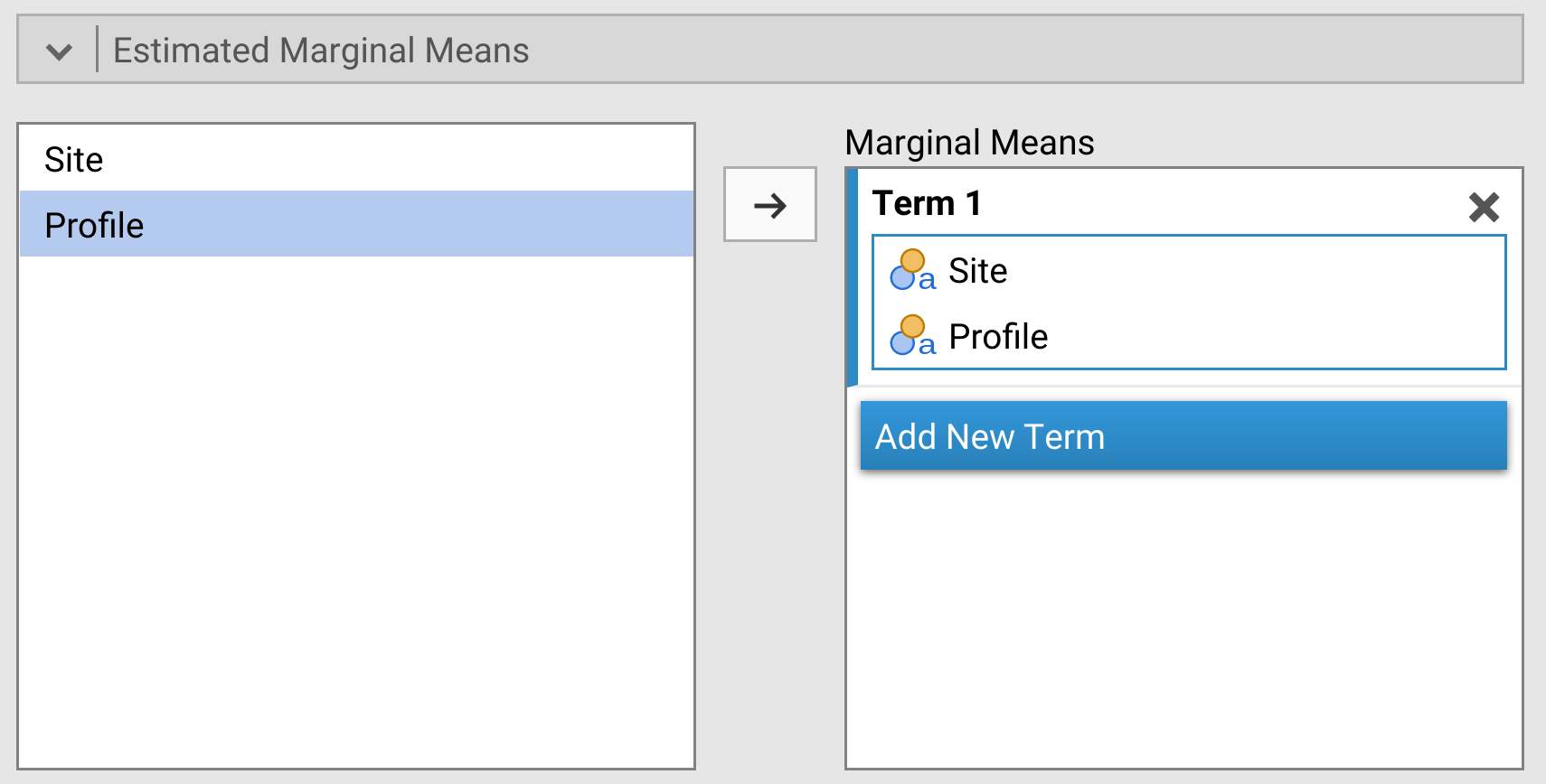
Figure 28.3: Jamovi two-way ANOVA test with the pull-down menu for Estimated Marginal Means, which will produce a plot showing the interaction effect of the two-way ANOVA.
In the panel on the right-hand side, a plot will appear under the heading ‘Estimated Marginal Means’. Based on what you learnt in Chapter 27 about interaction effects, what can you say about the interaction between Site and Profile? Does one Profile, in particular, appear to be causing the interaction to be significant? How can you infer this from the Estimated Marginal Means plot?
Try running a two-way ANOVA to test the effects of Site and Profile on Phosphorus concentration. Based on the ANOVA output, what can you conclude?