Chapter 35 Randomisation
Since introducing statistical hypothesis testing in Chapter 21, this book has steadily introduced statistical tests that can be run for different data types. In all of these statistical tests, the general idea is the same. We calculate some test statistic, then compare this test statistic to a predetermined null distribution to find the probability (i.e., p-value) of getting a test statistic as or more extreme than the one we calculated if the null hypothesis were true. This chapter introduces a different approach. Instead of using a pre-determined null distribution, we will build the null distribution using our data. This approach is not one that is often introduced in introductory statistics texts. It is included here for two reasons. First, randomisation presents a different way of thinking statistically without introducing an entirely different philosophical or methodological approach such as likelihood (Edwards, 1972) or Bayesian statistics (Lee, 1997). Second, it helps reinforce the concept of what null hypothesis testing is and what p-values are. Before explaining the randomisation approach, it is useful to summarise the parametric hypothesis tests introduced in earlier chapters.
35.1 Summary of parametric hypothesis testing
For the parametric tests introduced in previous chapters, null distributions included the t-distribution, F-distribution, and \(\chi^{2}\) distribution. For the t-tests in Chapter 22, the test statistic was the t-statistic, which we compared to a t-distribution. The one-sample t-test compared the mean of some variable (\(\bar{x}\)) to a specific number (\(\mu_{0}\)), the independent samples t-test compared two group means, and the paired samples t-test compared the mean difference between two paired groups. All of these tests used the t-distribution and calculated some value of t. Very low or high values of t at the extreme ends of the t-distribution are unlikely if the null hypothesis is true, so, in a two-tailed test, these are associated with low p-values that lead us to reject the null hypothesis.
For the analysis of variance (ANOVA) tests of Chapter 24, the relevant test statistic was the \(F\) statistic, with the F-distribution being the null distribution expected if two variances are equal. The one-way ANOVA used the within and among group variances of two or more groups to test the null hypothesis that all group means are equal. The two-way ANOVA of Chapter 27 extended the framework of the one-way ANOVA, allowing for a second variable of groups. This made it possible to simultaneously test whether or not the means of two different group types were the same, and whether or not there was an interaction between group types. All of these ANOVA tests calculated some value of \(F\) and compared it to the F distribution with appropriate degrees of freedom. Sufficiently high \(F\) values were associated with a low p-value and therefore the rejection of the null hypothesis.
The Chi-square tests introduced in Chapter 29 were used to test the frequencies of categorical observations and determine if they matched some expected frequencies (Chi-square goodness of fit test) or were associated in some way with the frequencies of another variable (Chi-square test of association). In these tests, the \(\chi^{2}\) statistic was used and compared to a null \(\chi^{2}\) distribution with an appropriate degrees of freedom. High \(\chi^{2}\) values were associated with low p-values and the rejection of the null hypothesis.
For testing the significance of correlation coefficients (see Chapter 30) and linear regression coefficients (see Chapter 32), a t-distribution was used. And an F distribution was used to test for the overall significance of linear regression models.
For these tests, the approach to hypothesis testing was therefore always to use the t-distribution, F distribution, or \(\chi^{2}\) distribution in some way. These distributions are more formally defined in mathematical statistics (Miller & Miller, 2004), a field of study that uses mathematics to derive the probability distributions that arise from an outcome of random events (e.g., the coin-flipping of Section 15.1). The reason that we use these distributions in statistical hypothesis testing is that they are often quite good at describing the outcomes that we expect when we collect a sample from a population. But this is not always the case. Recall that sometimes the assumptions of a particular statistical test were not met. In this case, a non-parametric alternative was introduced. The non-parametric test used the ranks of data instead of the actual values (e.g., Wilcoxon, Mann-Whitney U, Kruskal-Wallis H, and Spearman’s rank correlation coefficient tests). Randomisation uses a different approach.
35.2 Randomisation approach
Randomisation takes a different approach to null hypothesis testing. Instead of assuming a theoretical null distribution against which we compare our test statistic, we ask, ‘if the ordering of the data we collected was actually random, then what is the probability of getting a test statistic as or more extreme than the one that we actually did’. Rather than using a null distribution derived from mathematical statistics, we will build the null distribution by randomising our data in some useful way (Manly, 2007). Conceptually, this is often easier to understand because randomisation approaches make it easier to see why the null distribution exists and what it is doing. Unfortunately, these methods are more challenging to implement in practice because using them usually requires knowing a bit of coding. The best way to get started is with an instructive example.
35.3 Randomisation for hypothesis testing
As in several previous chapters, the dataset used here is inspired by the many species of wasps that lay their eggs in the flowers of the Sonoran Desert rock fig (Ficus petiolaris). This tree is distributed throughout the Baja peninsula, and in parts of mainland Mexico. Fig trees and the wasps that develop inside of them have a fascinating ecology, but for now we will just focus on the morphologies of two closely related species as an example. The fig wasps in Figure 35.1 are two unnamed species of the genus Idarnes, which we can refer to simply as ‘Short-ovipositor 1’ (SO1) and ‘Short-ovipositor 2’ (SO2).
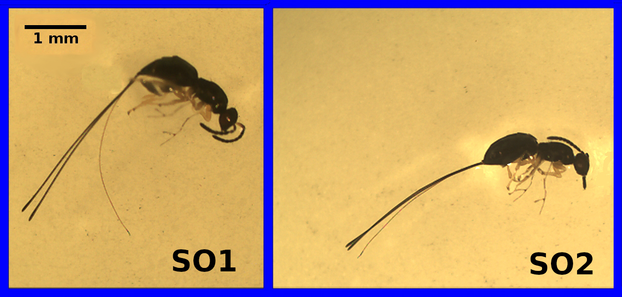
Figure 35.1: Two fig wasp species, roughly 3 mm in length, labelled ‘SO1’ and ‘SO2’. Image modified from Duthie, Abbott, and Nason (2015).
The reason that these two species are called ‘SO1’ and ‘SO2’ is that there is actually another species that lays its eggs in F. petiolaris flowers, one with an ovipositor that is at least twice as long as those in Figure 35.1 (Duthie et al., 2015).
Suppose that we have some data on the lengths of the ovipositors from each species. We might want to know whether the mean ovipositor length differs between the two species. Figure 35.2 shows histograms of ovipositor lengths collected from 32 fig wasps, 17 SO1s and 15 SO2s.
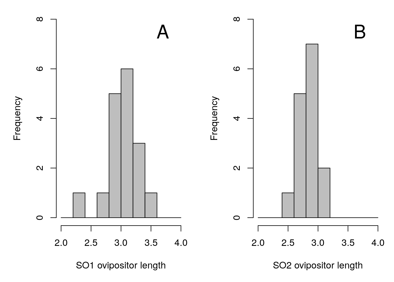
Figure 35.2: Ovipositor length distributions for two unnamed species of fig wasps, SO1 (A) and SO2 (B), collected from Baja, Mexico.
To test whether or not mean ovipositor length is different between these two fig wasps, our standard approach would be to use an independent samples t-test (see Section 22.2). The null hypothesis would be that the two means are the same, and the alternative (two-sided) hypothesis would be that the two means are not the same. We would need to check the assumption that the data are normally distributed, and that both samples have similar variances. Assuming that the assumption of normality is not violated (in which case we would need to consider a Mann-Whitney U test), and that both groups had similar variances (if not, we would use Welch’s t-test), we could proceed with calculating our t-statistic for pooled sample variance,
\[t_{\bar{y}_{\mathrm{SO1}} - \bar{y}_{\mathrm{SO2}}} = \frac{\bar{y}_{\mathrm{SO1}} - \bar{y}_{\mathrm{SO2}}}{s_{p}}.\]
The \(s_{p}\) is just being used as a short-hand to indicate the pooled standard deviation. For the two species of fig wasps, \(\bar{y}_{\mathrm{SO1}} =\) 3.0301176, \(\bar{y}_{\mathrm{SO2}} =\) 2.8448667, and \(s_{p} =\) 0.0765801. We can therefore calculate \(t_{\bar{y}_{\mathrm{SO1}} - \bar{y}_{\mathrm{SO2}}}\),
\[t_{\bar{y}_{\mathrm{SO1}} - \bar{y}_{\mathrm{SO2}}} = \frac{3.03 - 2.845}{0.077}.\]
After we calculate our t-statistic as \(t_{\bar{y}_{\mathrm{SO1}} - \bar{y}_{\mathrm{SO2}}} =\) 2.419, we would use the t-distribution to find the p-value (or, rather, get jamovi to do this for us). Figure 35.3 shows the t-distribution for 30 degrees of freedom with an arrow pointing at the value of \(t_{\bar{y}_{\mathrm{SO1}} - \bar{y}_{\mathrm{SO2}}} =\) 2.419.
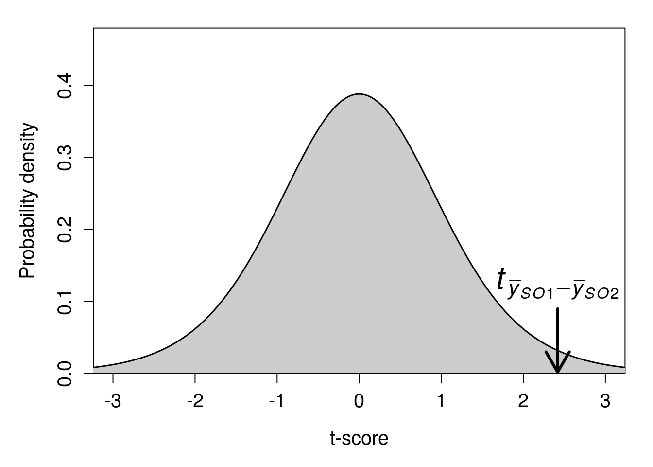
Figure 35.3: A t-distribution is shown with a calculated t-statistic of 2.419 indicated with a downward arrow.
If the null hypothesis is true, and \(\bar{y}_{\mathrm{SO1}}\) and \(\bar{y}_{\mathrm{SO2}}\) are actually sampled from a population with the same mean, then the probability of randomly sampling a value more extreme than 2.419 (i.e., greater than 2.419 or less than -2.419) is \(P =\) 0.0218352. We therefore reject the null hypothesis because \(P < 0.05\), and we conclude that the mean ovipositor lengths of each species are not the same.
Randomisation takes a different approach to the same problem. Instead of using the t-distribution in Figure 35.3, we will build our own null distribution using the fig wasp ovipositor length data. We do it by randomising group identity in the dataset. The logic is that if there really is no difference between group means, then we should be able to randomly shuffle group identities (species) and get a difference between means that is not far off the one we actually get from the data. In other words, what would the difference between group means be if we just mixed up all of the species (so some SO1s become SO2s, some SO2s become SO1s, some stay the same), then calculated the difference between means of the mixed up groups? If we just do this once, then we cannot learn much. But if we randomly shuffle the groups many, many times (say at least 9999), then we could see what the difference between group means would look like just by chance, i.e., if ovipositor length really was not different between SO1 and SO2. We could then compare our actual difference between mean ovipositor lengths to this null distribution in which the difference between groups means really is random (it has to be, we randomised the groups ourselves!). The idea is easiest to see using an interactive application82 that builds a null distribution of differences between the mean of SO1 and SO2 and compares it to the observed difference of \(\bar{y}_{\mathrm{SO1}} - \bar{y}_{\mathrm{SO2}} =\) 0.185.
With modern computing power, we do not need to do this randomisation manually. A desktop computer can easily reshuffle the species identities and calculate a difference between means thousands of times in less than a second. The histogram below shows the distribution of the difference between species mean ovipositor length if we were to randomly reshuffle groups 99999 times.
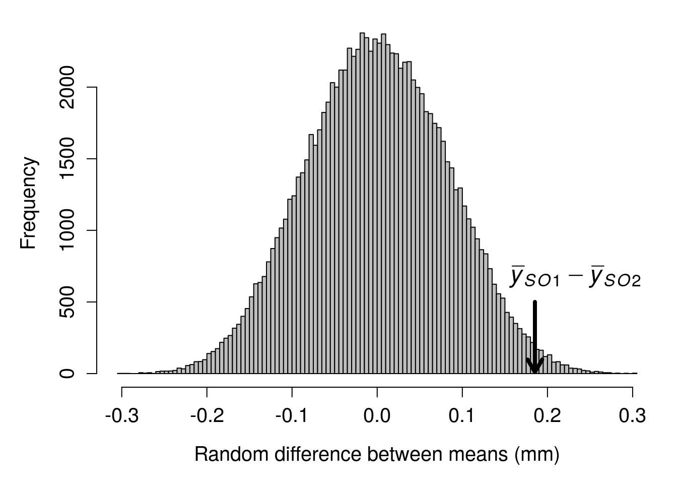
Figure 35.4: A distribution of the difference between mean species ovipositor lengths in two different species of fig wasps when species identity is randomly shuffled. The true difference between sampled mean SO1 and SO2 ovipositor lengths is pointed out with the black arrow at 0.185. Ovipositor lengths were collected from wasps in Baja, Mexico in 2010.
Given this distribution of randomised mean differences between species ovipositor lengths, the observed difference of 0.185 appears to be fairly extreme. We can quantify how extreme by figuring out the proportion of mean differences in the above histogram that are more extreme than our observed difference (i.e., greater than 0.185 or less than -0.185). It turns out that only 2085 out of 99999 random mean differences between ovipositor lengths were as or more extreme than our observed difference of 0.185. To express this as a probability, we can simply take the number of differences as or more extreme than our observed difference (including the observed one itself), divided by the total number of differences (again, including the observed one),
\[P = \frac{2085 + 1}{99999 + 1}.\]
When we calculate the above, we get a value of 0.02086. Notice that the calculated value is assigned with a ‘\(P\)’. This is because the value is a p-value (technically, an unbiased estimate of a p-value). Consider how close it is to the value of \(P =\) 0.0218352 that we got from the traditional t-test. Conceptually, we are doing the same thing in both cases; we are comparing a test statistic to a null distribution to see how extreme the differences between groups really are.
35.4 Randomisation assumptions
Recall from Section 22.4 the assumptions underlying t-tests, which include (1) data are continuous, (2) sample observations are a random sample from the population, and (3) sample means are normally distributed around the true mean. With randomisation, we do not need to assume 2 or 3. The randomisation approach is still valid even if the data are not normally distributed. Samples can have different variances. The observations do not even need to be independent. The validity of the randomisation approach even when standard assumptions do not apply can be quite useful.
The downside of the randomisation approach is that the statistical inferences that we make are limited to our sample, not the broader population (recall the difference between a sample and population from Chapter 4). Because the randomisation method does not assume that the data are a random sample from the population of interest (as is the case for the traditional t-test), we cannot formally make an inference about the difference between populations from which the sample was made. This is not necessarily a problem in practice. It is only relevant in terms of the formal assumptions of the model. Once we run our randomisation test, it might be entirely reasonable to argue verbally that the results of our randomisation test can generalise to our population of interest. In other words, we can argue that the difference between groups in the sample reflects a difference in the populations from which the sample came (Ernst, 2004; Ludbrook & Dudley, 1998).
35.5 Bootstrapping
We can also use randomisation to calculate confidence intervals for a variable of interest. Remember from Chapter 18 the traditional way to calculate lower and upper confidence intervals using a normal distribution,
\[LCI = \bar{x} - (z \times SE),\]
\[UCI = \bar{x} + (z \times SE).\]
Recall from Chapter 19 that a t-score is substituted for a z-score to account for a finite population size.
Suppose we want to calculate 95% confidence intervals for the ovipositor lengths of SO1 (Figure 35.2A). There are 17 ovipositor lengths for SO1.
3.256, 3.133, 3.071, 2.299, 2.995, 2.929, 3.291, 2.658, 3.406, 2.976, 2.817, 3.133, 3.000, 3.027, 3.178, 3.133, 3.210
To get the 95% confidence interval using the method from Chapter 18, we would calculate the mean \(\bar{x}_{SO1} =\) 3.03, standard deviation \(s_{\mathrm{SO1}} =\) 0.26, and the t-score for \(df = N - 1\) (where \(N = 17\)), which is \(t = 2.120\). Keeping in mind the formula for standard error \(s/\sqrt{N}\), we can calculate,
\[LCI = 3.03 - \left(2.120 \times \frac{0.26}{\sqrt{17}}\right),\]
\[UCI = 3.03 + \left(2.120 \times \frac{0.26}{\sqrt{17}}\right).\]
Calculating the above gives us values of LCI = 2.896 and UCI = 3.164.
Again, randomisation uses a different approach to get an estimate of the same confidence intervals. Instead of calculating the standard error and multiplying it by a z-score or t-score to encompass a particular interval of probability density, we can instead resample the data we have with replacement many times, calculating the mean each time we resample. The general idea is that this process of resampling approximates what would happen if we were to go back and resample new data from our original population many times, thereby giving us the distribution of means from all of these hypothetical resampling events (Manly, 2007). To calculate our 95% confidence intervals, we then only need to rank the calculated means and find the mean closest to the lowest 2.5% and the highest 97.5%.
Remember from Section 15.3 that the phrase ‘resampling with replacement’ just means that we are going to randomly sample some values, but not remove them from the pool of possible values after they are sampled. If we resample the numbers above with replacement, we might therefore sample some values two or more times by chance, and other values might not be sampled at all. The numbers below resample from the above with replacement.
2.299, 3.027, 2.929, 3.256, 3.071, 2.658, 3.133, 3.027, 2.976, 2.817, 3.406, 3.210, 2.976, 3.133, 3.133, 3.178, 2.299
Notice that some values appear more than once in the data above, while other values that were present in the original dataset are no longer present after resampling with replacement. Consequently, these new resampled data have a different mean than the original. The mean of the original 17 SO1 ovipositor length values was 3.03, and the mean of the values resampled above is 2.972. We can resample another set of numbers to get a new mean.
3.133, 3.027, 2.658, 3.291, 3.133, 2.299, 2.976, 2.658, 2.929, 3.133, 2.929, 2.995, 3.071, 2.299, 3.000, 3.133, 3.133
The mean of the above sample is 2.929. We can continue doing this until we have a high number of random samples and means. Figure 35.5 shows the distribution of means if we repeat this process of resampling with replacement and calculating the mean 10000 times.
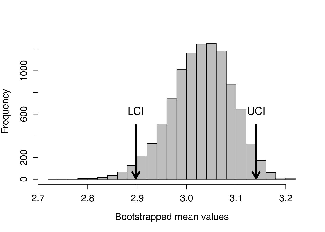
Figure 35.5: A distribution of bootstrapped values of ovipositor lengths from 17 measurements of a fig wasp species collected from Baja, Mexico. A total of 10000 bootstrapped means are shown, and arrows indicate the location of the 2.5% (LCI) and 97.5% (UCI) ranked boostrapped mean values.
The arrows show the locations of the 2.5% and 97.5% ranked values of the bootstrapped means. Note that it does not matter if the above distribution is not normal (it appears a bit skewed). The bootstrap still works. The values using the randomisation approach are LCI = 2.897 and UCI = 3.14. These values are quite similar to those calculated with the traditional approach because we are doing the same thing, conceptually. But instead of finding confidence intervals of the sample means around the true mean using the t-distribution, we are actually simulating the process of resampling from the population and calculating sample means many times.
35.6 Randomisation conclusions
The examples demonstrated in this chapter are just a small set of what is possible using randomisation approaches. Randomisation and bootstrapping are highly flexible tools that can be used in a variety of ways (Manly, 2007). They could be used as substitutes (or complements) to any of the hypothesis tests that we have used in this book. For example, to use a randomisation approach for testing whether or not a correlation coefficient is significantly different from 0, we could randomly shuffle the values of one variable 9999 times. After each shuffle, we would calculate the Pearson product moment correlation coefficient, then use the 9999 randomised correlations as a null distribution to compare against the observed correlation coefficient. This would give us a plot like the one shown in Figure 35.4, but showing the null distribution of the correlation coefficient instead of the difference between group means. Similar approaches could be used for ANOVA or linear regression (Manly, 2007).