Chapter 23 Practical. Hypothesis testing and t-tests
This chapter focuses on applying the concepts about hypothesis testing from Chapter 21 and the statistical tests from Chapter 22 in jamovi (The jamovi project, 2024). There will be five exercises in total, which will focus on using t-tests and their non-parametric equivalents. The data for this chapter focus on an example of biology and environmental sciences education. Similar to the example in Chapter 22, it uses datasets of student test scores (note that these data are entirely fictional; I have not used scores from real students). We will use 2022 test data52 and 2023 test data53. Variables in these datasets include scores from three different tests.
23.1 One sample t-test
First, we will consider test data from 2022. Open this dataset in jamovi. Before doing any analysis, compute a new column of data called ‘Overall’ that is each student’s mean test score. To do this, double-click on the fifth column of data, then when a new panel opens up, choose ‘NEW COMPUTED VARIABLE’ from the list of available options. Your input should look like Figure 23.1.
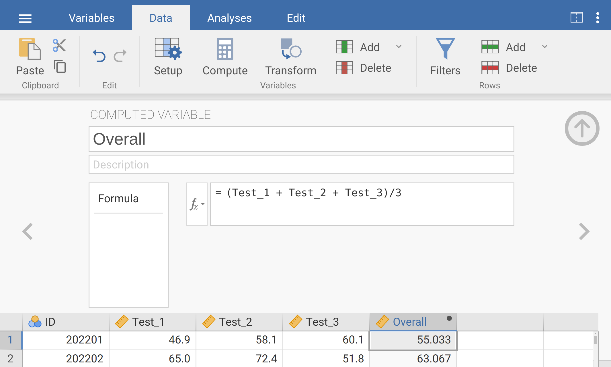
Figure 23.1: Jamovi interface for adding a new computed variable called ‘Overall’ and calculating the mean of the three tests.
After calculating the overall grade for each student, find the sample size (\(N\)), overall sample mean (\(\bar{x}\)), and sample standard deviation (\(s\)). Report these below.
\(N =\) __________________
\(\bar{x} =\) _______________
\(s =\) ___________________
Suppose that you have been told that the national average of overall student test scores in classes like yours is \(\mu_{0} = 60.1\). A concerned colleague approaches you and expresses concern that your test scores are lower than the national average. You decide to test whether or not your students’ scores really are lower than the national average, or if your colleague’s concerns are unfounded. What kind(s) of statistical test would be most appropriate to use in this case, and what is the null hypothesis (\(H_{0}\)) of the test?
Test to use: ___________________________
\(H_{0}\): _______________________
What is the alternative hypothesis (\(H_{A}\)), and should you use a one- or two-tailed test?
\(H_{A}\): _______________________
One- or two-tailed? __________________________
To test if the mean of overall student scores in your class is significantly lower than \(\mu_{0} = 60.1\) (technically, that your student’s scores were sampled from a population with a mean lower than 60.1), we might use a one-tailed, one sample t-test. Recall from Section 22.4 the assumptions underlying a t-test:
- Data are continuous (i.e., not count or categorical data)
- Sample observations are a random sample from the population
- Sample means are normally distributed around the true mean
We will first focus on the first and third assumption. First, the sample data are indeed continuous. But are the sample means normally distributed around the true mean? A sufficient condition to fulfil this assumption is that the sample data are normally distributed (Johnson, 1995; Lumley et al., 2002). We can test whether or not the overall mean student scores are normally distributed. In the jamovi toolbar, find the button that says ‘T-Tests’ (second from the left), then choose ‘One Sample T-test’ from the pull-down menu. A new window will open up. In a one sample t-test, there is only one dependent variable, which in this case is ‘Overall’. Move the variable ‘Overall’ to the Dependent Variables box with the right arrow. Below the boxes, find the checkbox options under ‘Assumption Checks’. Check both ‘Normality test’ (this is a Shapiro-Wilk test of normality) and ‘Q-Q Plot’.
After checking the box for ‘Normality test’ and ‘Q-Q Plot’, new output will appear in the panel on the right-hand side. The first output is a table showing the results of a Shapiro-Wilk test. The Shapiro-Wilk test tests the null hypothesis that the dependent variable is normally distributed (note, this is not our t-test yet; we use the Shapiro-Wilk test to see if the assumptions of the t-test are violated or not). If we reject the null hypothesis, then we will conclude that the data are not normally distributed. If we do not reject the null hypothesis, then we will assume that the data are normally distributed. From the Normality Test table, what is the p-value of the Shapiro-Wilk test?
\(P\) = _____________________
Based on this p-value, should we reject the null hypothesis? ______________
Now have a look at the Q-Q plot. This plot can also be used to assess whether or not the data are normally distributed. If the data are normally distributed, then the points in the Q-Q plot should fall roughly along the diagonal black line. These plots take some practice to read and interpret, but for now, just have a look at the Q-Q plot and think about how it relates to the results of the Shapiro-Wilk test of normality. It might be useful to plot a histogram of the overall scores too in order to judge whether or not they are normally distributed (most researchers will use both a visual inspection of the data and a normality test to evaluate whether or not the assumption of normality is satisfied).
Assuming that we have not rejected our null hypothesis, we can proceed with our one sample t-test. To do this, make sure the variable ‘Overall’ is still in the Dependent Variables box, then make sure the check box ‘Student’s’ is checked below Tests. Underneath Hypothesis, change the test value to 60.1 (because \(\mu_{0} = 60.1\)) and put the radio button to ‘< Test value’ to test the null hypothesis that the mean overall score of students is the same as \(\mu_{0}\) against the alternative hypothesis that it is less than \(\mu_{0}\). On the right panel of jamovi, you will see a table with the t-statistic, degrees of freedom, and p-value of the one sample t-test. Write these values down below.
t-statistic: _________________
degrees of freedom: __________________
p-value: ____________________
Remember how the t-statistic, degrees of freedom, and p-value are all related. Based on the p-value, should you reject the null hypothesis that your students’ mean overall grade is the same as the national average? Why or why not?
Based on this test, how would you respond to your colleague who is concerned that your students are performing below the national average?
Consider again the three assumptions of the t-test listed above. Is there an assumption that might be particularly suspect when comparing the scores of students in a single classroom with a national average? Why or why not?
We will now test whether students in this dataset improved their test scores from Test 1 to Test 2.
23.2 Paired t-test
Suppose we want to test whether or not students in this dataset improved their grades from Test 1 to Test 2. In this case, we are interested in the variables ‘Test_1’ and ‘Test_2’, but we are not just interested in whether or not the means of the two test scores are the same. Instead, we want to know if the scores of individual students increased or not. The data are therefore naturally paired. Each test score belongs to a unique student, and each student has a score for Test 1 and Test 2. To test whether or not there has been an increase in test scores, go to the ‘T-Tests’ button in the jamovi toolbar and select ‘Paired Samples T-Test’ from the pull-down menu. Place ‘Test_1’ in the Paired Variables box first, followed by ‘Test_2’. Jamovi will interpret the first variable placed in the box as ‘Measure 1’, and the second variable placed in the box as ‘Measure 2’. Before looking at any test results, first check to see if the difference between Test 1 and Test 2 scores is normally distributed using the same Assumption Checks as in the previous exercise. Is there any reason to believe that the data are not normally distributed?
We want to know if student grades have improved. What is the null hypothesis (\(H_{0}\)) and alternative hypothesis (\(H_{A}\)) in this case?
\(H_{0}\): _____________________
\(H_{A}\): _____________________
To test the null hypothesis against the appropriate alternative hypothesis, select the radio button ‘Measure 1 < Measure 2’. As with the one sample t-test, on the right panel of jamovi, you will see a table with the t-statistic, degrees of freedom, and p-value of the one sample t-test. Write these values down below.
t-statistic: _________________
degrees of freedom: __________________
p-value: ____________________
Based on this p-value, should you reject or fail to reject your null hypothesis? What can you then conclude about student test scores?
Note that this paired t-test is, mathematically, the exact same as a one sample t-test. If you want to convince yourself of this, you can create a new computed variable that is \(Test\:1 - Test\:2\), then run a one sample t-test. You will see that the t-statistic, degrees of freedom, and p-value are all the exact same. Next, we will consider a case in which the assumption of normality is violated.
23.3 Wilcoxon test
Suppose that we want to test the null hypothesis that the scores from Test 3 of the dataset used in Exercises 23.1 and 23.2 were sampled from a population with a mean of \(\mu_{0} = 62\). We are not interested in whether the scores are higher or lower than 62, just that they are different. Consequently, what should our alternative hypothesis (\(H_{A}\)) be?
\(H_{A}\): ___________________
Use the same procedure that you did in Exercise 23.1 to test this new hypothesis concerning Test 3 scores. First, check the assumption that the Test 3 scores are normally distributed. What is the p-value of the Shapiro-Wilk test this time?
\(P\) = ____________________
What inference can you make from the Q-Q plot? Do the points fall along the diagonal line?
Based on the Shapiro-Wilk test and Q-Q plot, is it safe to assume that the Test 3 scores are normally distributed?
Since the Test 3 scores are not normally distributed (and an assumption of the t-test is therefore violated), we can use the non-parametric Wilcoxon signed-rank test instead, as was introduced in Section 22.5.1. To apply the Wilcoxon test, check the box ‘Wilcoxon rank’ under the Tests option. Next, make sure to set the ‘Test value’ to 62 under the Hypothesis option. What are the null and alternative hypotheses of this test?
\(H_{0}\): _______________________
\(H_{A}\): _______________________
The results of the Wilcoxon signed-rank test will appear in the ‘One Sample T-Test’ table in the right panel of jamovi in a row called ‘Wilcoxon W’. What is the test statistic (not the p-value) for the Wilcoxon test?
Test statistic: __________________
Based on what you learnt in Section 22.5.1, what does this test statistic actually mean?
Now look at the p-value for the Wilcoxon test. What is the p-value, and what should you conclude from it?
\(P\) = _______________
Conclusion: ___________________
Next, we will introduce a new dataset to test hypotheses concerning the means of two different groups.
23.4 Independent samples t-test
In the first three exercises, we tested hypotheses using data from 2022. In this exercise, we will test the differences in mean test scores between students from 2022 and 2023. As might be expected, the 2022 and 2023 datasets are stored in separate files. What we need to do first is combine the data into a single tidy dataset. To do this, open the Year 2 dataset in a spreadsheet and copy all of the data (but not the column names). You can then paste these data directly into jamovi in the next available row (row 22). Next, add in a new column for ‘Year’, so that you can differentiate 2022 students from 2023 students in the same dataset. To do this, you can right-click on the ‘ID’ column and choose ‘Add Variable’, then ‘Insert’. A new column will appear to the left, which you can name ‘Year’. Input ‘2022’ for rows 1–21, then ‘2023’ for the remaining rows that you just pasted into jamovi (see Figure 23.2).
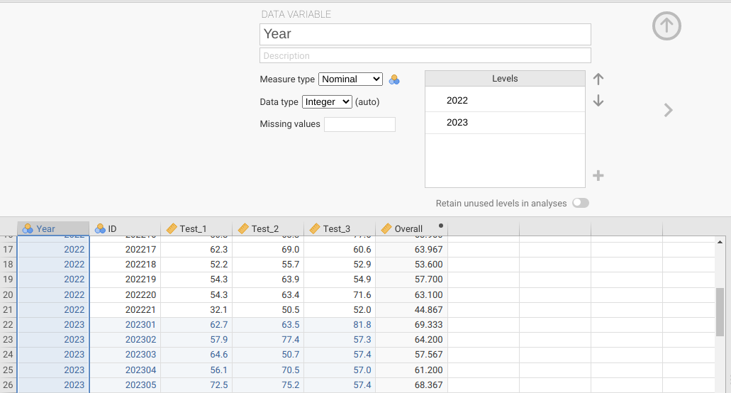
Figure 23.2: Jamovi interface for inserting a new variable called ‘Year’, and the value 2022 pasted into the first 21 rows. The value 2023 has been pasted into the remaining rows of the ‘Year’ column.
Note that ‘Year’ does not necessarily need to be in the first column. You could have added it in as the second column, or as the last (i.e., the location of the column will not affect any analyses).
With the new data now included in jamovi, we can compare student test scores between years. Suppose that we first want to test the null hypothesis that the overall student scores have the same mean, \(\mu_{2022} = \mu_{2023}\), against the alternative hypothesis that \(\mu_{2022} \neq \mu_{2023}\). Is this a one- or a two-tailed hypothesis?
One- or two-tailed? _________________
It is generally a good idea to plot and summarise your data before running any statistical tests. If you have time, have a look at histograms of the Overall student scores from each year, and look at some summary statistics from the Descriptives output. This will give you a sense of what to expect when running your test diagnostics (e.g., tests of normality) and might alert you to any problems before actually running the analysis (e.g., major outliers that do not make sense, such as a student having an overall score of over 1000 due to a data input error).
After you have had a look at the histograms and summary statistics, go to the jamovi toolbar and navigate to ‘T-Tests’, then the ‘Independent Samples T-Test’ from the pull-down menu. Remember that our objective here is to test whether the means of two groups (2022 versus 2023) are the same. We can therefore place the ‘Overall’ variable in the Dependent Variables box, then ‘Year’ in the Grouping Variable box. Before running the independent samples t-test, we again need to check our assumptions. In addition to the assumption of normality that we checked for in the previous exercises, recall from Section 22.2 that the standard Student’s independent samples t-test also assumes that the variances of groups (i.e., 2022 and 2023 scores) are the same, while the Welch’s t-test does not assume equal variances. In addition to the Assumption Checks options ‘Normality test’ and ‘Q-Q plot’, there is also now a test called ‘Homogeneity test’, which will test the null hypothesis that groups have the same variances (Figure 23.3). This is called a ‘Levene’s test’, and we can interpret it in a similar way to the Shapiro-Wilk test of normality.
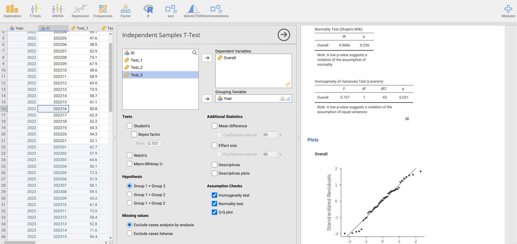
Figure 23.3: Jamovi interface for running the assumptions of an Independent Samples T-Test. Here, we are testing if the Overall grades of students differ by Year (2022 versus 2023). Assumption Checks include a test for homogeneity of variances (Homogeneity test) and normal distribution of Overall grades (Normality test and Q-Q plot).
If our p-value is sufficiently low (\(P < 0.05\)), then we reject the null hypothesis that the groups have the same variances. Based on the Assumption Checks in jamovi (and Figure 23.3), what can you conclude about the t-test assumptions?
What is the p-value for the Levene’s test?
\(P\) = _________________
It appears from our test of assumptions that we do not reject the null hypothesis that the data are normally distributed, but we should reject the null hypothesis that the groups have equal variances. Based on what you learnt in Section 22.2, what is the appropriate test to run in this case?
Test: ____________________
Note that the appropriate test should be available as a check box underneath the Tests options. Check the box for the correct test, then report the test statistic and p-value from the table that appears in the right panel.
Test statistic: ____________________
\(P\) = __________________
What can you conclude from this t-test?
Next, we will compare mean Test 3 scores between years 2022 and 2023.
23.5 Mann-Whitney U Test
Suppose that we now want to use the data from the previous exercise to test whether or not Test 3 scores differ between years. Consequently, in this exercise, Test 3 will be our Dependent Variable and Year will again be the Grouping Variable (also called the ‘Independent variable’). Below, summarise the hypotheses for this new test.
\(H_{0}:\) ________________
\(H_{A}:\) ________________
Is this a one- or two-tailed test? _____________
Next, begin a new Independent Samples T-Test in jamovi and check the assumptions underlying the t-test. Do the variances appear to be the same for Test 3 scores in 2022 versus 2023? How can you make this conclusion?
Next, check to see if the data are normally distributed. What is the p-value of the Shapiro-Wilk test?
\(P\) = ________________
Now, have a look at the Q-Q plot. What can you infer from this plot about the normality of the data, and why?
Based on what you found from testing the model assumptions above, and the material in Chapter 22, what test is the most appropriate one to use?
Test: ________________
Run the above test in jamovi, then report the test statistic and p-value below.
Test statistic: ____________
\(P =\) ___________
Based on what you learnt in Section 22.5.2, what does this test statistic actually mean?
Finally, what conclusions can you make about Test 3 scores in 2022 versus 2023?
I have not introduced an example in which a transformation (such as a log transformation) is applied to normalise a dataset, as explained in Section 22.4. To do such a transformation, you could create a new computed variable in jamovi and calculate it as the natural log (LN) of a variable (e.g., Test 3). Figure 23.4 illustrates what this should look like.
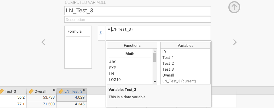
Figure 23.4: Jamovi interface for creating a new computed variable that is the natural logarithm of Test 3 data scores in a fictional dataset of student grades.
Lastly, suppose that you wanted to test whether students from 2023 improved their scores from Test 1 to Test 2 more than students from 2022 did. Is there a way to do this with just the tools presented here and in Chapter 22? Think about how the paired t-test works, and how you could apply that logic to test for the difference in the change between two independent samples (2022 versus 2023). What could you do to test the null hypothesis that the change in scores from Test 1 to Test 2 is the same between years?