23 Data wrangling—continued
23.2 Introduction
This chapter revisits the process of data wrangling with some additional techniques.
23.2.1 ungroup()
When we use a group_by() and summarize() pairing, we can calculate summary statistics for each group in our data.
In this example, we calculate the difference in a country’s life expectancy from the continent’s mean life expectancy - for example, the difference in 2007 between life expectancy in Canada and the mean life expectancy of countries in the Americas
What we had seen before was the use of group_by() |> summarize() to create summary statistics by a group:
## # A tibble: 5 × 2
##   continent lifeExp_mean
##   <fct>            <dbl>
## 1 Africa            54.8
## 2 Americas          73.6
## 3 Asia              70.7
## 4 Europe            77.6
## 5 Oceania           80.7
But how can we compare the Canada value to the Americas mean shown here? One strategy would be to join this table to the original, using “continent” as the key value.
But there is another solution: group_by() |> mutate()
Step 1:
Filter for 2007
Then group by continent and
Mutate to get the mean continental life expectancy
Note: the tibble that results from this retains the “Groups:”. It is important to be aware of this, since any future manipulations of this table will be based on that grouping.
gm_life_2007 <-
gapminder |>
  # select and filter
  select(country, continent, year, lifeExp) |>
  filter(year == 2007) |>
  # group_by |> mutate
  group_by(continent) |>
  mutate(lifeExp_con_mean = mean(lifeExp))

gm_life_2007
## # A tibble: 142 × 5
## # Groups: continent [5]
## country continent year lifeExp lifeExp_con_mean
## <fct> <fct> <int> <dbl> <dbl>
## 1 Afghanistan Asia 2007 43.8 70.7
## 2 Albania Europe 2007 76.4 77.6
## 3 Algeria Africa 2007 72.3 54.8
## 4 Angola Africa 2007 42.7 54.8
## 5 Argentina Americas 2007 75.3 73.6
## 6 Australia Oceania 2007 81.2 80.7
## 7 Austria Europe 2007 79.8 77.6
## 8 Bahrain Asia 2007 75.6 70.7
## 9 Bangladesh Asia 2007 64.1 70.7
## 10 Belgium Europe 2007 79.4 77.6
## # ℹ 132 more rowsTo that data frame, we can append another mutate to calculate the difference between the individual country and the continent.
Note that addition of the the ungroup() function, which removes the grouping.
In the resulting table, we see the observations for 2007, with all the countries in the Americas. Note that they all have the same value of “lifeExp_con_mean”, which is subtracted from “lifeExp” to get the “lifeExp_diff” variable. Countries which have a life expectancy above the continental mean show positive values, while those where the life expectancy is below, have negative values.
gm_life_2007 |>
  ungroup() |>
  # subtract continent mean from individual country
  mutate(lifeExp_diff = lifeExp - lifeExp_con_mean) |>
  # select and filter for just the Americas
  filter(continent == "Americas")
## # A tibble: 25 × 6
## country continent year lifeExp lifeExp_con_mean lifeExp_diff
## <fct> <fct> <int> <dbl> <dbl> <dbl>
## 1 Argentina Americas 2007 75.3 73.6 1.71
## 2 Bolivia Americas 2007 65.6 73.6 -8.05
## 3 Brazil Americas 2007 72.4 73.6 -1.22
## 4 Canada Americas 2007 80.7 73.6 7.04
## 5 Chile Americas 2007 78.6 73.6 4.94
## 6 Colombia Americas 2007 72.9 73.6 -0.719
## 7 Costa Rica Americas 2007 78.8 73.6 5.17
## 8 Cuba Americas 2007 78.3 73.6 4.66
## 9 Dominican Republic Americas 2007 72.2 73.6 -1.37
## 10 Ecuador Americas 2007 75.0 73.6 1.39
## # ℹ 15 more rowsIn the version below, it’s a single pipe that uses both year and continent as the grouping variables. This gets the same result with the added comparison of the individual country to the world average for that year, for every year in the data:
gm_life <- gapminder |>
  # select
  select(country, continent, year, lifeExp) |>
  # continent life expectancy
  group_by(year, continent) |>
  mutate(lifeExp_con_mean = mean(lifeExp)) |>
  ungroup() |>
  mutate(lifeExp_con_diff = lifeExp - lifeExp_con_mean) |>
  # world life expectancy
  group_by(year) |>
  mutate(lifeExp_earth_mean = mean(lifeExp)) |>
  ungroup() |>
  mutate(lifeExp_earth_diff = lifeExp - lifeExp_earth_mean)

gm_life |>
  filter(year == 2007 & continent == "Americas")
## # A tibble: 25 × 8
## country continent year lifeExp lifeExp_con_mean lifeExp_con_diff lifeExp_earth_mean
## <fct> <fct> <int> <dbl> <dbl> <dbl> <dbl>
## 1 Argentina Americas 2007 75.3 73.6 1.71 67.0
## 2 Bolivia Americas 2007 65.6 73.6 -8.05 67.0
## 3 Brazil Americas 2007 72.4 73.6 -1.22 67.0
## 4 Canada Americas 2007 80.7 73.6 7.04 67.0
## 5 Chile Americas 2007 78.6 73.6 4.94 67.0
## 6 Colombia Americas 2007 72.9 73.6 -0.719 67.0
## 7 Costa Rica Americas 2007 78.8 73.6 5.17 67.0
## 8 Cuba Americas 2007 78.3 73.6 4.66 67.0
## 9 Dominican Republic Americas 2007 72.2 73.6 -1.37 67.0
## 10 Ecuador Americas 2007 75.0 73.6 1.39 67.0
## # ℹ 15 more rows
## # ℹ 1 more variable: lifeExp_earth_diff <dbl>Now we can create a plot to compare Canada to the averages of the continent and the world over time:
gm_life |>
  filter(country == "Canada") |>
ggplot() +
  geom_line(aes(x = year, y = lifeExp_con_diff), colour = "red") +
  geom_line(aes(x = year, y = lifeExp_earth_diff), colour = "blue")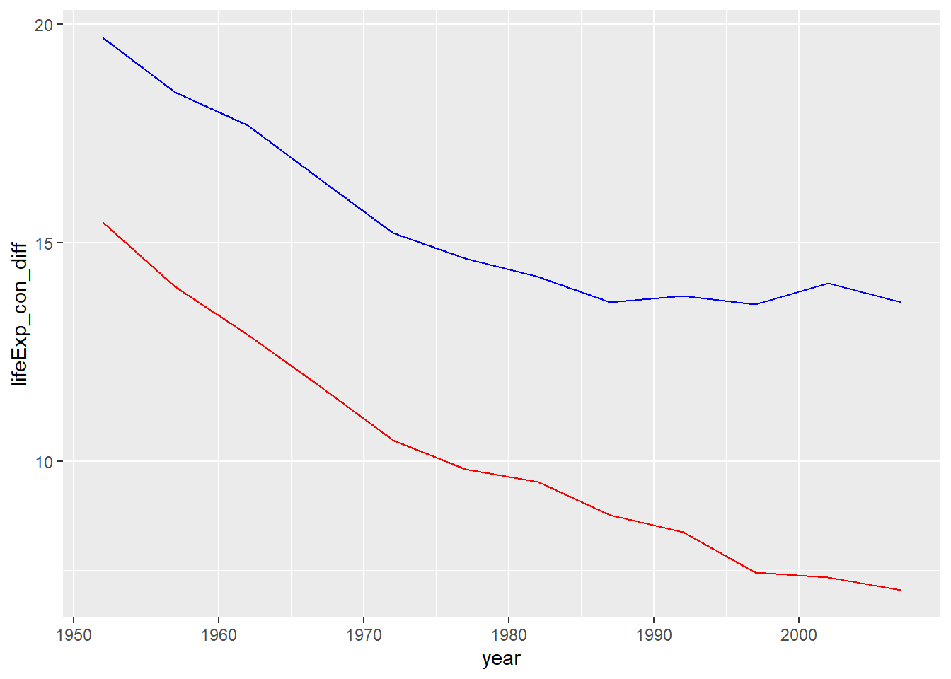
This isn’t a story about Canada’s life expectancy getting worse—life expectancy in Canada improved from 68.8 in 1952 to 80.7 in 2007.
What the chart shows are the substantial improvements in the life expectancy for people elsewhere around the world (the blue line) and in the Americas (the red line). While life expectancy in Canada improved and remains well above average, for many countries of the world, life expectancy is much, much longer than it was 70 years ago.
23.2.1.1 Moneyball data
A similar approach was used to create the “pay_index” variable in the Moneyball assignment.
First, we read the data in the file:
mlb_pay_wl <- read_csv("data/mlb_pay_wl_original.csv")
mlb_pay_wl
## # A tibble: 630 × 6
## year_num tm attend_g est_payroll w l
## <dbl> <chr> <dbl> <dbl> <dbl> <dbl>
## 1 1999 ANA 27816 55633166 70 92
## 2 1999 ARI 37280 68703999 100 62
## 3 1999 ATL 40554 73341000 103 59
## 4 1999 BAL 42385 80805863 78 84
## 5 1999 BOS 30200 64097500 94 68
## 6 1999 CHC 34739 62343000 67 95
## 7 1999 CHW 16529 25820000 75 86
## 8 1999 CIN 25137 33962761 96 67
## 9 1999 CLE 42820 73679962 97 65
## 10 1999 COL 42976 61935837 72 90
## # ℹ 620 more rowsYou will see that the file contains the team payroll, wins and losses, but not the two calculated variables that we used in the linear regression model.
To replicate the file we used in the assignment, we need to add
- a win-loss percentage
# win-loss percentage is the number of wins, divided by the total number of games played
mlb_pay_wl <- mlb_pay_wl |>
  mutate(wl_pct = round(w / (w + l), 3))

mlb_pay_wl
## # A tibble: 630 × 7
## year_num tm attend_g est_payroll w l wl_pct
## <dbl> <chr> <dbl> <dbl> <dbl> <dbl> <dbl>
## 1 1999 ANA 27816 55633166 70 92 0.432
## 2 1999 ARI 37280 68703999 100 62 0.617
## 3 1999 ATL 40554 73341000 103 59 0.636
## 4 1999 BAL 42385 80805863 78 84 0.481
## 5 1999 BOS 30200 64097500 94 68 0.58
## 6 1999 CHC 34739 62343000 67 95 0.414
## 7 1999 CHW 16529 25820000 75 86 0.466
## 8 1999 CIN 25137 33962761 96 67 0.589
## 9 1999 CLE 42820 73679962 97 65 0.599
## 10 1999 COL 42976 61935837 72 90 0.444
## # ℹ 620 more rows- the pay index, comparing the individual team payroll to the average of all the teams that season, where 100 is the league average.
Note that this requires a group/ungroup within the pipe.
mlb_pay_wl <- mlb_pay_wl |>
  group_by(year_num) |>
  mutate(league_avg_pay = mean(est_payroll)) |>
  ungroup() |>
  mutate(pay_pct_league = est_payroll / league_avg_pay * 100)

mlb_pay_wl
## # A tibble: 630 × 9
## year_num tm attend_g est_payroll w l wl_pct league_avg_pay pay_pct_league
## <dbl> <chr> <dbl> <dbl> <dbl> <dbl> <dbl> <dbl> <dbl>
## 1 1999 ANA 27816 55633166 70 92 0.432 50119642. 111.
## 2 1999 ARI 37280 68703999 100 62 0.617 50119642. 137.
## 3 1999 ATL 40554 73341000 103 59 0.636 50119642. 146.
## 4 1999 BAL 42385 80805863 78 84 0.481 50119642. 161.
## 5 1999 BOS 30200 64097500 94 68 0.58 50119642. 128.
## 6 1999 CHC 34739 62343000 67 95 0.414 50119642. 124.
## 7 1999 CHW 16529 25820000 75 86 0.466 50119642. 51.5
## 8 1999 CIN 25137 33962761 96 67 0.589 50119642. 67.8
## 9 1999 CLE 42820 73679962 97 65 0.599 50119642. 147.
## 10 1999 COL 42976 61935837 72 90 0.444 50119642. 124.
## # ℹ 620 more rowsLet’s create a histogram to show the distribution of team payroll, relative to the league average:
mlb_pay_wl |>
  ggplot(aes(x = pay_pct_league)) +
    geom_histogram()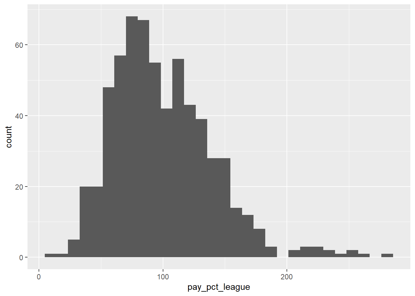
23.2.2 across()
The across() function:
makes it easy to apply the same transformation to multiple columns, allowing you to use select() semantics inside in “data-masking” functions like summarise() and mutate(). See
These examples are variations of the ones from the {dplyr} reference “Apply a function (or functions) across multiple columns”. That resource, and the related vignette “colwise” have more examples and details.
For our examples, we will use the penguins data table from the {palmerpenguins} package.
library(palmerpenguins)

penguins
## # A tibble: 344 × 8
## species island bill_length_mm bill_depth_mm flipper_length_mm body_mass_g sex year
## <fct> <fct> <dbl> <dbl> <int> <int> <fct> <int>
## 1 Adelie Torgersen 39.1 18.7 181 3750 male 2007
## 2 Adelie Torgersen 39.5 17.4 186 3800 female 2007
## 3 Adelie Torgersen 40.3 18 195 3250 female 2007
## 4 Adelie Torgersen NA NA NA NA <NA> 2007
## 5 Adelie Torgersen 36.7 19.3 193 3450 female 2007
## 6 Adelie Torgersen 39.3 20.6 190 3650 male 2007
## 7 Adelie Torgersen 38.9 17.8 181 3625 female 2007
## 8 Adelie Torgersen 39.2 19.6 195 4675 male 2007
## 9 Adelie Torgersen 34.1 18.1 193 3475 <NA> 2007
## 10 Adelie Torgersen 42 20.2 190 4250 <NA> 2007
## # ℹ 334 more rowsIn this example, the rounding function is applied to the two bill measurements:
## # A tibble: 344 × 8
##    species island    bill_length_mm bill_depth_mm flipper_length_mm body_mass_g sex     year
##    <fct>   <fct>              <dbl>         <dbl>             <int>       <int> <fct>  <int>
##  1 Adelie  Torgersen             39            19               181        3750 male    2007
##  2 Adelie  Torgersen             40            17               186        3800 female  2007
##  3 Adelie  Torgersen             40            18               195        3250 female  2007
##  4 Adelie  Torgersen             NA            NA                NA          NA <NA>    2007
##  5 Adelie  Torgersen             37            19               193        3450 female  2007
##  6 Adelie  Torgersen             39            21               190        3650 male    2007
##  7 Adelie  Torgersen             39            18               181        3625 female  2007
##  8 Adelie  Torgersen             39            20               195        4675 male    2007
##  9 Adelie  Torgersen             34            18               193        3475 <NA>    2007
## 10 Adelie  Torgersen             42            20               190        4250 <NA>    2007
## # ℹ 334 more rows
Since those measures are of type “double” and the other two numeric measures are integer, we could identify the variables we want to round using the type, via the is.double argument:
## # A tibble: 344 × 8
##    species island    bill_length_mm bill_depth_mm flipper_length_mm body_mass_g sex     year
##    <fct>   <fct>              <dbl>         <dbl>             <int>       <int> <fct>  <int>
##  1 Adelie  Torgersen             39            19               181        3750 male    2007
##  2 Adelie  Torgersen             40            17               186        3800 female  2007
##  3 Adelie  Torgersen             40            18               195        3250 female  2007
##  4 Adelie  Torgersen             NA            NA                NA          NA <NA>    2007
##  5 Adelie  Torgersen             37            19               193        3450 female  2007
##  6 Adelie  Torgersen             39            21               190        3650 male    2007
##  7 Adelie  Torgersen             39            18               181        3625 female  2007
##  8 Adelie  Torgersen             39            20               195        4675 male    2007
##  9 Adelie  Torgersen             34            18               193        3475 <NA>    2007
## 10 Adelie  Torgersen             42            20               190        4250 <NA>    2007
## # ℹ 334 more rows
It’s also possible to use the across() function to apply the same function(s) to multiple variables. Here we will use the group-by() |> summarize() functions to calculate the mean of the bill measurements.
Note also the
starts_with()function that is used to identify the columns of interest.The
mean()function has a tilde in front. In R, the “~” is used to indicate a function, so
~mean(.x, na.rm = TRUE)
is a shortcut for
function(.x){mean(x, na.rm = TRUE)} where “.x” is a placeholder for every variable we have defined in our across() function.
(It might help to think of this like a looping function—for every variable, the summarise() loops through the mean() function.)
penguins |>
  group_by(species) |>
  summarise(across(starts_with("bill_"),
                   ~mean(.x, na.rm = TRUE)))
## # A tibble: 3 × 3
## species bill_length_mm bill_depth_mm
## <fct> <dbl> <dbl>
## 1 Adelie 38.8 18.3
## 2 Chinstrap 48.8 18.4
## 3 Gentoo 47.5 15.0In this example, the list argument defines a list of functions to be applied. By putting the name of the function ahead of the function (e.g. mean = mean), that term gets appended to the name of the variables created by the summarise() function. (You may want to see what happens when you change this to mean, sd or cat = mean, dog = sd!)
penguins |>
  group_by(species) |>
  summarise(across(starts_with("bill_"),
                   list(mean = mean, sd = sd),
                   na.rm = TRUE))
## # A tibble: 3 × 5
## species bill_length_mm_mean bill_length_mm_sd bill_depth_mm_mean bill_depth_mm_sd
## <fct> <dbl> <dbl> <dbl> <dbl>
## 1 Adelie 38.8 2.66 18.3 1.22
## 2 Chinstrap 48.8 3.34 18.4 1.14
## 3 Gentoo 47.5 3.08 15.0 0.98123.2.3 Calculations across rows
Another common data manipulation outcome we seek is the average across our variables…so far everything we’ve done has been down the variables. R is really good at the latter. Here’s some techniques to apply a function across a row.
(This is drawn from the {dplyr} vignette “Row-wise operations”)
First we create a little tibble:
df <- tibble(x = 1:2, y = 3:4, z = 5:6)
df
## # A tibble: 2 × 3
## x y z
## <int> <int> <int>
## 1 1 3 5
## 2 2 4 6Then we apply the rowwise() function:
df |> rowwise()## # A tibble: 2 × 3
## # Rowwise:
## x y z
## <int> <int> <int>
## 1 1 3 5
## 2 2 4 6It looks just the same, but you will note the “Rowwise:” indicator above the table. This means that any functions that are applied will run across the rows instead of the usual columnwise direction.
## # A tibble: 2 × 4
## # Rowwise:
##       x     y     z     m
##   <int> <int> <int> <dbl>
## 1     1     3     5     3
## 2     2     4     6     4
Without the rowwise() function we get 3.5 for both rows. This the mean of “x” and “y” and “z” (that is, the mean of the integers 1 through 6):
## # A tibble: 2 × 4
##       x     y     z     m
##   <int> <int> <int> <dbl>
## 1     1     3     5   3.5
## 2     2     4     6   3.5
In the examples below, we will use a bigger tibble:
df2 <- tibble(id = letters[1:6], w = 10:15, x = 20:25, y = 30:35, z = 40:45)
df2
## # A tibble: 6 × 5
## id w x y z
## <chr> <int> <int> <int> <int>
## 1 a 10 20 30 40
## 2 b 11 21 31 41
## 3 c 12 22 32 42
## 4 d 13 23 33 43
## 5 e 14 24 34 44
## 6 f 15 25 35 45To calculate the sum of the columns, we could mutate() to get a new column, or summarize() for just the total.
By putting the “id” in the rowwise() function, it acts as a grouping variable across the rows.
## # A tibble: 6 × 6
## # Rowwise:  id
##   id        w     x     y     z total
##   <chr> <int> <int> <int> <int> <int>
## 1 a        10    20    30    40   100
## 2 b        11    21    31    41   104
## 3 c        12    22    32    42   108
## 4 d        13    23    33    43   112
## 5 e        14    24    34    44   116
## 6 f 15 25 35 45 120## # A tibble: 6 × 2
## # Groups: id [6]
## id total
## <chr> <int>
## 1 a 100
## 2 b 104
## 3 c 108
## 4 d 112
## 5 e 116
## 6 f 120To streamline the specification of the variables we use, the c_across() function can be applied, indicating the range of the variables we want to sum and average:
## # A tibble: 6 × 3
## # Groups:   id [6]
##   id    total average
##   <chr> <int>   <dbl>
## 1 a       100      25
## 2 b       104      26
## 3 c       108      27
## 4 d       112      28
## 5 e       116      29
## 6 f       120      30
There are two other functions that streamline this syntax still further: rowSums and rowMeans.
Note: this function has the rowwise() built in!
## # A tibble: 6 × 6
##   id        w     x     y     z total
##   <chr> <int> <int> <int> <int> <dbl>
## 1 a        10    20    30    40   100
## 2 b        11    21    31    41   104
## 3 c        12    22    32    42   108
## 4 d        13    23    33    43   112
## 5 e        14    24    34    44   116
## 6 f        15    25    35    45   120
23.2.4 Comparing values between rows
It is common in time series analysis to compare values that are in different rows. For example, in a data table with quarterly revenue data, you might want to report on the change from one quarter to the next. Or with monthly data where there is a strong seasonal trend comparing one month to the next might not be all that useful (think of the difference in retail sales in January compared to December), so a comparison to the same month of the previous year would reveal more insight. The New Housing Price Index example we saw earlier incorporates both month-over-month and year-over-year comparisions.
The {dplyr} package has two functions, lag() and lead(), that allow us access to the value in a different row.
23.2.4.1 Exercies:
Using the {gapminder} data, find the country with biggest jump in life expectancy (between any two consecutive records) for each continent.
# One of many solutions
gapminder |>
  group_by(country) |>
  mutate(prev_lifeExp = lag(lifeExp),
         jump = lifeExp - prev_lifeExp) |>
  arrange(desc(jump), continent)
## # A tibble: 1,704 × 8
## # Groups: country [142]
## country continent year lifeExp pop gdpPercap prev_lifeExp jump
## <fct> <fct> <int> <dbl> <int> <dbl> <dbl> <dbl>
## 1 Cambodia Asia 1982 51.0 7272485 624. 31.2 19.7
## 2 China Asia 1967 58.4 754550000 613. 44.5 13.9
## 3 Rwanda Africa 1997 36.1 7212583 590. 23.6 12.5
## 4 Rwanda Africa 2002 43.4 7852401 786. 36.1 7.33
## 5 Mauritius Africa 1957 58.1 609816 2034. 51.0 7.10
## 6 Bulgaria Europe 1957 66.6 7651254 3009. 59.6 7.01
## 7 El Salvador Americas 1987 63.2 4842194 4140. 56.6 6.55
## 8 China Asia 1957 50.5 637408000 576. 44 6.55
## 9 Myanmar Asia 1957 41.9 21731844 350 36.3 5.59
## 10 Albania Europe 1962 64.8 1728137 2313. 59.3 5.54
## # ℹ 1,694 more rows
# Another solution
gapminder |>
  group_by(country) |>
  mutate(prev_lifeExp = lag(lifeExp),
         jump = lifeExp - prev_lifeExp) |>
  ungroup() |>
  group_by(continent) |>
  slice(which.max(jump)) |>
  arrange(desc(jump))
## # A tibble: 5 × 8
## # Groups: continent [5]
## country continent year lifeExp pop gdpPercap prev_lifeExp jump
## <fct> <fct> <int> <dbl> <int> <dbl> <dbl> <dbl>
## 1 Cambodia Asia 1982 51.0 7272485 624. 31.2 19.7
## 2 Rwanda Africa 1997 36.1 7212583 590. 23.6 12.5
## 3 Bulgaria Europe 1957 66.6 7651254 3009. 59.6 7.01
## 4 El Salvador Americas 1987 63.2 4842194 4140. 56.6 6.55
## 5 New Zealand Oceania 1992 76.3 3437674 18363. 74.3 2.01
# Another solution
gapminder |>
  group_by(country) |>
  mutate(prev_lifeExp = lag(lifeExp),
         jump = lifeExp - prev_lifeExp) |>
  ungroup() |>
  group_by(continent) |>
  slice_max(jump) |>
  arrange(desc(jump))
## # A tibble: 5 × 8
## # Groups: continent [5]
## country continent year lifeExp pop gdpPercap prev_lifeExp jump
## <fct> <fct> <int> <dbl> <int> <dbl> <dbl> <dbl>
## 1 Cambodia Asia 1982 51.0 7272485 624. 31.2 19.7
## 2 Rwanda Africa 1997 36.1 7212583 590. 23.6 12.5
## 3 Bulgaria Europe 1957 66.6 7651254 3009. 59.6 7.01
## 4 El Salvador Americas 1987 63.2 4842194 4140. 56.6 6.55
## 5 New Zealand Oceania 1992 76.3 3437674 18363. 74.3 2.01
23.3 Recode variables with case_when()
We sometimes find ourselves in a situation where we want to recode our existing variables into other categories. For example, sometimes you have a handful of categories that make up the bulk of the total, and summarizing the smaller categories into an “all other” makes the table or plot easier to read. Think of the populations of the 13 Canadian provinces and territories: the four most populous provinces (Ontario, Quebec, British Columbia, and Alberta) account for roughly 85% of the country’s population…the other 15% are spread across nine provinces and territories. We might want to show a table with only five rows, with the smallest nine provinces and territories grouped into a single row.
We can do this with a function in {dplyr}, case_when().
canpop <- read_csv("data/canpop.csv")
canpop
## # A tibble: 13 × 2
## province_territory population
## <chr> <dbl>
## 1 Ontario 13448494
## 2 Quebec 8164361
## 3 British Columbia 4648055
## 4 Alberta 4067175
## 5 Manitoba 1278365
## 6 Saskatchewan 1098352
## 7 Nova Scotia 923598
## 8 New Brunswick 747101
## 9 Newfoundland and Labrador 519716
## 10 Prince Edward Island 142907
## 11 Northwest Territories 41786
## 12 Nunavut 35944
## 13 Yukon 35874In this first solution, we name the largest provinces separately:
canpop |>
  mutate(pt_grp = case_when(
    # evaluation ~ new value
    province_territory == "Ontario" ~ "Ontario",
    province_territory == "Quebec" ~ "Quebec",
    province_territory == "British Columbia" ~ "British Columbia",
    province_territory == "Alberta" ~ "Alberta",
    # all others get recoded as "other"
    TRUE ~ "other"
  ))
## # A tibble: 13 × 3
## province_territory population pt_grp
## <chr> <dbl> <chr>
## 1 Ontario 13448494 Ontario
## 2 Quebec 8164361 Quebec
## 3 British Columbia 4648055 British Columbia
## 4 Alberta 4067175 Alberta
## 5 Manitoba 1278365 other
## 6 Saskatchewan 1098352 other
## 7 Nova Scotia 923598 other
## 8 New Brunswick 747101 other
## 9 Newfoundland and Labrador 519716 other
## 10 Prince Edward Island 142907 other
## 11 Northwest Territories 41786 other
## 12 Nunavut 35944 other
## 13 Yukon 35874 otherBut that’s a lot of typing. A more streamlined approach is to put the name of our provinces in a list, and then recode our new variable with the value from the original variable:
canpop |>
  mutate(pt_grp = case_when(
    province_territory %in% c("Ontario", "Quebec", "British Columbia", "Alberta") ~ province_territory,
    TRUE ~ "other"
  ))
## # A tibble: 13 × 3
## province_territory population pt_grp
## <chr> <dbl> <chr>
## 1 Ontario 13448494 Ontario
## 2 Quebec 8164361 Quebec
## 3 British Columbia 4648055 British Columbia
## 4 Alberta 4067175 Alberta
## 5 Manitoba 1278365 other
## 6 Saskatchewan 1098352 other
## 7 Nova Scotia 923598 other
## 8 New Brunswick 747101 other
## 9 Newfoundland and Labrador 519716 other
## 10 Prince Edward Island 142907 other
## 11 Northwest Territories 41786 other
## 12 Nunavut 35944 other
## 13 Yukon 35874 otherBut we can do even better, by using a comparison to create a population threshold:
canpop <- canpop |>
  mutate(pt_grp = case_when(
    population > 4000000 ~ province_territory,
    TRUE ~ "other"
  ))

canpop
## # A tibble: 13 × 3
## province_territory population pt_grp
## <chr> <dbl> <chr>
## 1 Ontario 13448494 Ontario
## 2 Quebec 8164361 Quebec
## 3 British Columbia 4648055 British Columbia
## 4 Alberta 4067175 Alberta
## 5 Manitoba 1278365 other
## 6 Saskatchewan 1098352 other
## 7 Nova Scotia 923598 other
## 8 New Brunswick 747101 other
## 9 Newfoundland and Labrador 519716 other
## 10 Prince Edward Island 142907 other
## 11 Northwest Territories 41786 other
## 12 Nunavut 35944 other
## 13 Yukon 35874 otherNow we can use that new variable to group a table:
## # A tibble: 5 × 2
##   pt_grp             pt_pop
##   <chr>               <dbl>
## 1 Ontario          13448494
## 2 Quebec            8164361
## 3 other             4823643
## 4 British Columbia  4648055
## 5 Alberta           4067175
In another example, we might want to group a series of dates by decade.
date_list <- tribble(
  ~ref_date,
  "2000-02-29",
  "2004-02-29",
  "2011-01-01",
  "2014-03-31",
  "2019-09-01",
  "2023-03-28"
) |>
  mutate(ref_date = ymd(ref_date))

date_list
## # A tibble: 6 × 1
## ref_date
## <date>
## 1 2000-02-29
## 2 2004-02-29
## 3 2011-01-01
## 4 2014-03-31
## 5 2019-09-01
## 6 2023-03-28To create the decade groupings, the case_when() follows a mutate() function. Note that we are using lubridate::year() to extract the year value for our comparison.
date_list <- date_list |>
  mutate(ref_decade = case_when(
    year(ref_date) < 2010 ~ "aughts",
    year(ref_date) < 2020 ~ "teens",
    TRUE ~ "other"
  ))

date_list
## # A tibble: 6 × 2
## ref_date ref_decade
## <date> <chr>
## 1 2000-02-29 aughts
## 2 2004-02-29 aughts
## 3 2011-01-01 teens
## 4 2014-03-31 teens
## 5 2019-09-01 teens
## 6 2023-03-28 otherAnother option for this problem would be to round the year value down to the nearest 10. This uses the round_any() function from the {plyr} package. (The round() function from base R rounds to the nearest 10, so a year like 2019 gets rounded up to the 2020s. The floor() function, related to round(), rounds down, but only to the nearest integer.)
# to round year value down to first year of the decade
date_list |>
  mutate(ref_decade = plyr::round_any(year(ref_date), accuracy = 10, f = floor))
## # A tibble: 6 × 2
## ref_date ref_decade
## <date> <dbl>
## 1 2000-02-29 2000
## 2 2004-02-29 2000
## 3 2011-01-01 2010
## 4 2014-03-31 2010
## 5 2019-09-01 2010
## 6 2023-03-28 202023.3.1 Multiple comparisons
In this example from the case_when() reference page:, it uses different combinations of three variables to create a single fourth variable. It uses the built-in data set “starwars”, a list of characters from the movies.
# case_when is particularly useful inside mutate when you want to
# create a new variable that relies on a complex combination of existing
# variables
starwars
## # A tibble: 87 × 14
## name height mass hair_color skin_color eye_color birth_year sex gender homeworld species
## <chr> <int> <dbl> <chr> <chr> <chr> <dbl> <chr> <chr> <chr> <chr>
## 1 Luke Skyw… 172 77 blond fair blue 19 male mascu… Tatooine Human
## 2 C-3PO 167 75 <NA> gold yellow 112 none mascu… Tatooine Droid
## 3 R2-D2 96 32 <NA> white, bl… red 33 none mascu… Naboo Droid
## 4 Darth Vad… 202 136 none white yellow 41.9 male mascu… Tatooine Human
## 5 Leia Orga… 150 49 brown light brown 19 fema… femin… Alderaan Human
## 6 Owen Lars 178 120 brown, gr… light blue 52 male mascu… Tatooine Human
## 7 Beru Whit… 165 75 brown light blue 47 fema… femin… Tatooine Human
## 8 R5-D4 97 32 <NA> white, red red NA none mascu… Tatooine Droid
## 9 Biggs Dar… 183 84 black light brown 24 male mascu… Tatooine Human
## 10 Obi-Wan K… 182 77 auburn, w… fair blue-gray 57 male mascu… Stewjon Human
## # ℹ 77 more rows
## # ℹ 3 more variables: films <list>, vehicles <list>, starships <list>For this example, we mutate a new variable based on whether a character is a robot, or whether they are large (defined by height or mass).
starwars |>
  select(name:mass, gender, species) |>
  mutate(
    type = case_when(
      species == "Droid"        ~ "robot",
      height > 150 | mass > 200 ~ "large",
      TRUE                      ~ "other"
    )
  )
## # A tibble: 87 × 6
## name height mass gender species type
## <chr> <int> <dbl> <chr> <chr> <chr>
## 1 Luke Skywalker 172 77 masculine Human large
## 2 C-3PO 167 75 masculine Droid robot
## 3 R2-D2 96 32 masculine Droid robot
## 4 Darth Vader 202 136 masculine Human large
## 5 Leia Organa 150 49 feminine Human other
## 6 Owen Lars 178 120 masculine Human large
## 7 Beru Whitesun lars 165 75 feminine Human large
## 8 R5-D4 97 32 masculine Droid robot
## 9 Biggs Darklighter 183 84 masculine Human large
## 10 Obi-Wan Kenobi 182 77 masculine Human large
## # ℹ 77 more rowsAnd order matters! The function case_when() finds all of the cases that meet the first criteria, and then applies the second criteria to the remaining observations. If we switch the order and move “robot” below “large”, we find (as one example) that C-3PO is now in the large category, as they are over 150 cm in height.
# create "type" variable
starwars |>
  select(name:mass, species) |>
  mutate(
    type = case_when(
      # large first, then robot
      height > 150 | mass > 200 ~ "large",
      species == "Droid"        ~ "robot",
      TRUE                      ~ "other"
    )
  )
## # A tibble: 87 × 5
## name height mass species type
## <chr> <int> <dbl> <chr> <chr>
## 1 Luke Skywalker 172 77 Human large
## 2 C-3PO 167 75 Droid large
## 3 R2-D2 96 32 Droid robot
## 4 Darth Vader 202 136 Human large
## 5 Leia Organa 150 49 Human other
## 6 Owen Lars 178 120 Human large
## 7 Beru Whitesun lars 165 75 Human large
## 8 R5-D4 97 32 Droid robot
## 9 Biggs Darklighter 183 84 Human large
## 10 Obi-Wan Kenobi 182 77 Human large
## # ℹ 77 more rows-30-