Assignment 3 - week 4 - Moneyball
The book Moneyball: The Art of Winning an Unfair Game (and the movie of the same name) tells the story of the 2002 Oakland Athletics baseball team. That year, the team won 103 of its 162 games (a win-loss percentage12 of 0.636). Only the New York Yankees had a better record that Major League Baseball (MLB) season; the Yankees also won 103 but played one fewer due to a rain-out, so finished with a win-loss percentage of 0.640.
Oakland had a payroll of $40 million (only Tampa Bay and Montreal, at $34.4 and $38.7 million, were lower). The Yankees, by contrast, had the highest payroll at $125.9 million, with a roster full of star players.
Another way to compare an individual team’s payroll is relative to the Major League Baseball average. The Yankees payroll was 186% of the league average—for every 100 dollars the average team spent, the Yankees spent $186. The next closest team in spending was the Boston Red Sox, whose salary bill was 160% of the league average at $108 million. Oakland, by contrast, spent 59% of the league average—while the average team spent $100 dollars, the Athletics were constrained to spending $60.
And yet these two teams—one packed with highly-paid star players, and the other staffed with players that other teams had cast off—managed to have very similar and enormously successful seasons.
It’s a great story. Part of the drama is about how the Atheltics started using data analysis to identify those players who were undervalued in the market.

Let’s use the tidyverse packages and some elements in base R to explore the relationship between payroll spending and team success.
The first thing we’ll do is read in the data file. For this we will use “mlb_pay_wl.csv”.13
mlb_pay_wl <- read_csv("data/mlb_pay_wl.csv")This file has a record (observation) for each of the Major League Baseball (MLB) teams for the seasons 1999 through 2019. This is 630 rows of data.
For each team season, the file has
the attendance per game (“attend_g”)
the estimated payroll (“est_payroll”)
the pay as a percent of the league (“pay_index”), where 100 is the league average for that year. A value of 110 would be 10 percent higher than the league average for the season; a value of 90 would be 10 percent lower.
wins and losses (“w” and “l”); counts of the number of games won and lost in that season. Note that the Major League Baseball season is 162 games long, but the sum of wins and losses isn’t always 162. Sometimes teams play fewer because of cancellations due to weather, and they might play an extra game at the end of the season to determine which team will advance to the playoffs.
and the winning percentage (“w_l_percent”) where 0.500 represents winning as many games as losing. The highest value in this period was the Seattle Mariners, whose win-loss “percentage” was 0.716 (71.6%) in 2001 (116 of 162 games). The worst team in the data was the Detroit Tigers in 2003, who lost 119 of their 162 games (a percentage of 0.265).
mlb_pay_wl## # A tibble: 630 × 8
## year_num tm attend_g est_payroll pay_index w l w_l_percent
## <dbl> <chr> <dbl> <dbl> <dbl> <dbl> <dbl> <dbl>
## 1 1999 ANA 27816 55633166 111. 70 92 0.432
## 2 1999 ARI 37280 68703999 137. 100 62 0.617
## 3 1999 ATL 40554 73341000 146. 103 59 0.636
## 4 1999 BAL 42385 80805863 161. 78 84 0.481
## 5 1999 BOS 30200 64097500 128. 94 68 0.58
## 6 1999 CHC 34739 62343000 124. 67 95 0.414
## 7 1999 CHW 16529 25820000 51.5 75 86 0.466
## 8 1999 CIN 25137 33962761 67.8 96 67 0.589
## 9 1999 CLE 42820 73679962 147. 97 65 0.599
## 10 1999 COL 42976 61935837 124. 72 90 0.444
## # ℹ 620 more rowsVisualizing the data
For our exercise, we will explore the relationship between payroll and wins. Does paying star players always lead to success?
Or phrased another way, can we predict team success based on the team payroll? In this case, the win-loss percentage is the dependent variable, while team payroll (as a percent of the league average) is the independent variable.
First, let’s create a scatterplot to visualize the relationship. We will put payroll on the X axis, and win-loss percent on the Y.
ggplot(mlb_pay_wl, aes(x = pay_index, y = w_l_percent)) +
  geom_point()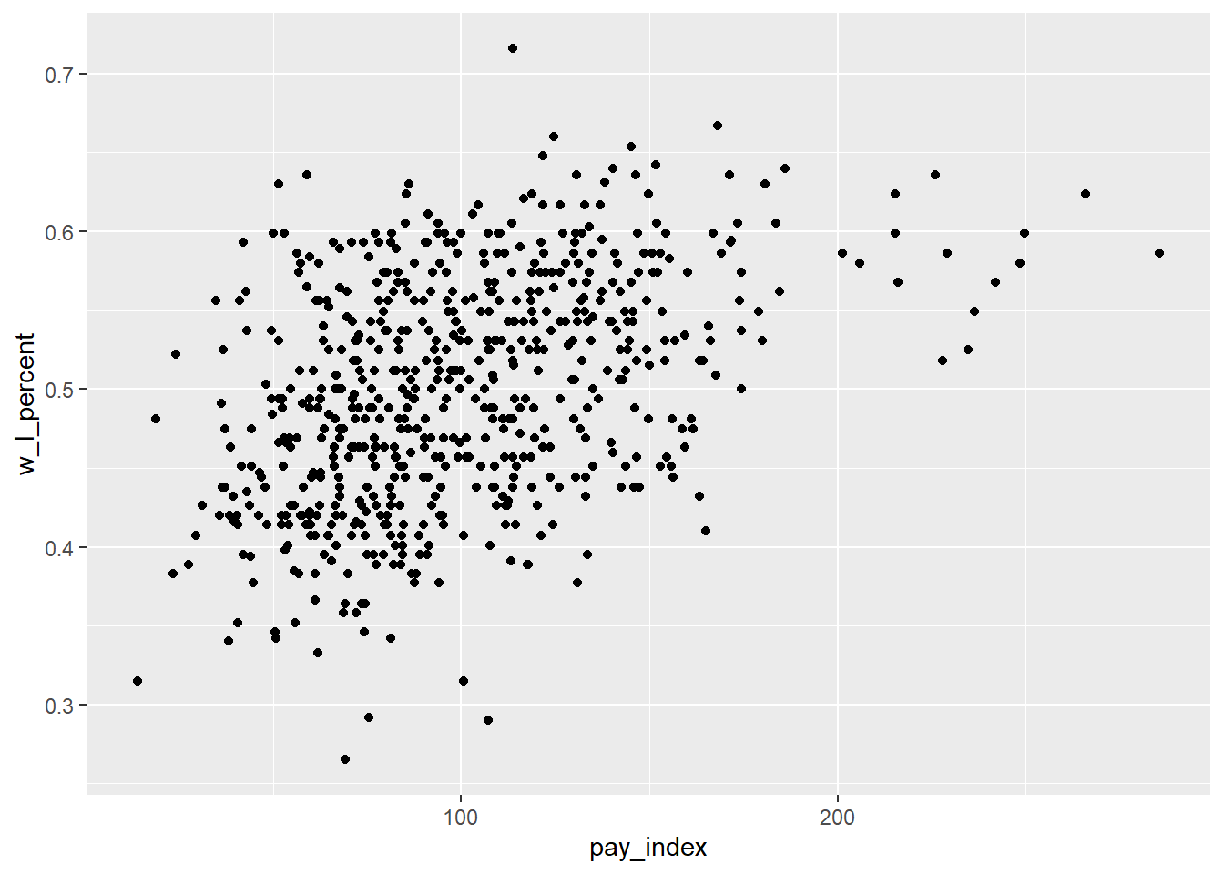
That’s a lot of points on our plot. To help us navigate, in the plot below there are two lines on the plot.
The red line runs vertically at the “1” point on the X axis. The teams to the left of the line spent below the league average for that season; the teams to the right spent more. As you can see, there have been cases when some teams spent twice as much as the league average.
The blue line runs horizontally at the “0.5” point on the Y axis. Above this line, the teams won more games than they lost. Below the line, they lost more games than they won.
ggplot(mlb_pay_wl, aes(x = pay_index, y = w_l_percent)) +
  geom_point() +
  geom_vline(xintercept  = 100, colour = "red", size = 2) +
  geom_hline(yintercept = 0.5, colour = "blue", size = 2)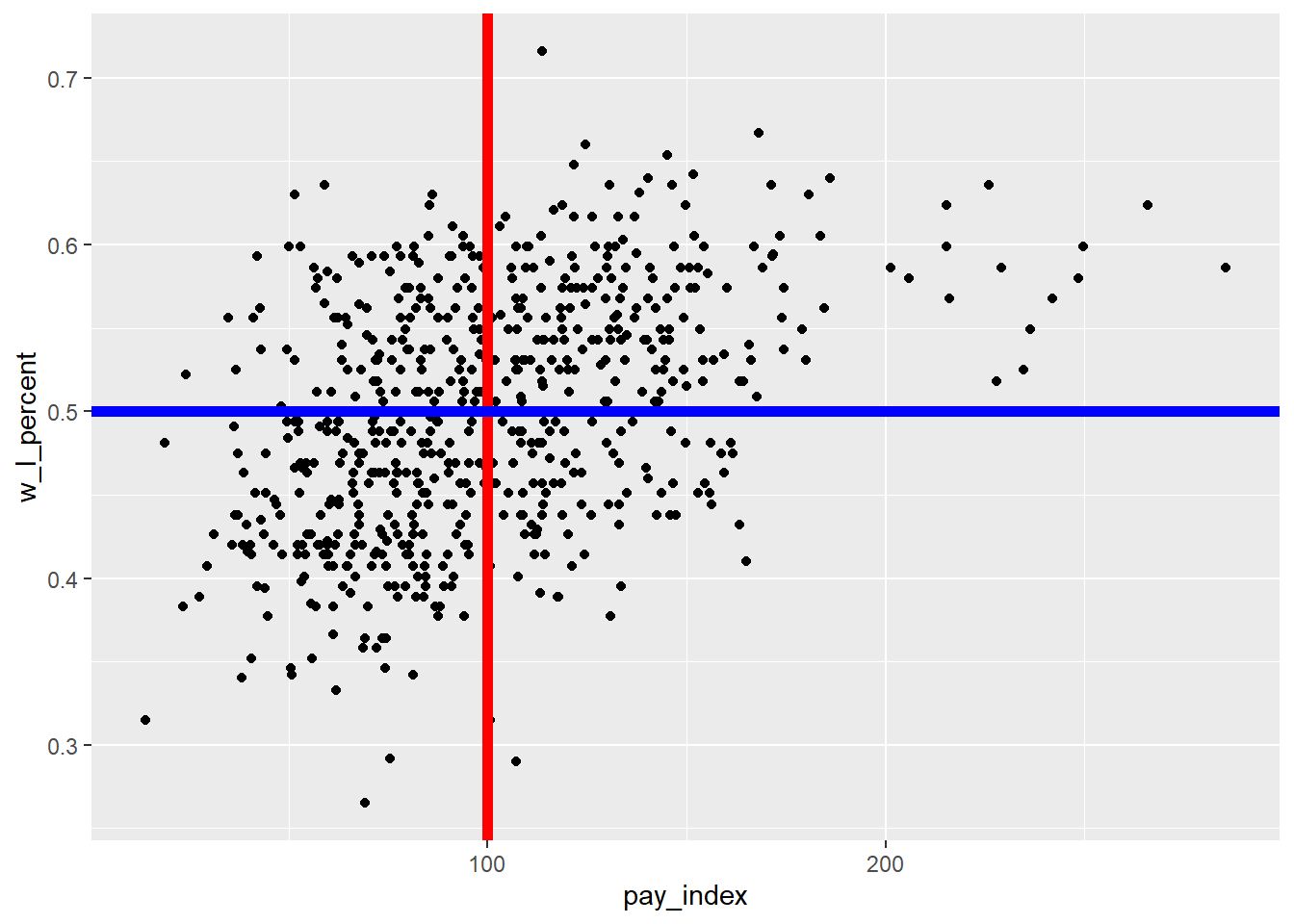
Based on a quick glance, there seems to be more high payroll teams in the top right quadrant (high payroll plus winning season) than bottom right (high payroll plus losing season). By contrast, there might be a few more low payroll teams with losing seasons than low payroll teams with winning seasons.
Let’s use our regression modeling skills to see if there’s a consistent relationship with paying star players lots of money, and winning lots of games.
First, we can visualize the relationship using the geom_smooth(method = lm) function. The “method = lm” part refers to a linear model—that is to say, a regression model.
ggplot(mlb_pay_wl, aes(x = pay_index, y = w_l_percent)) +
  geom_point() +
  geom_smooth(method = lm)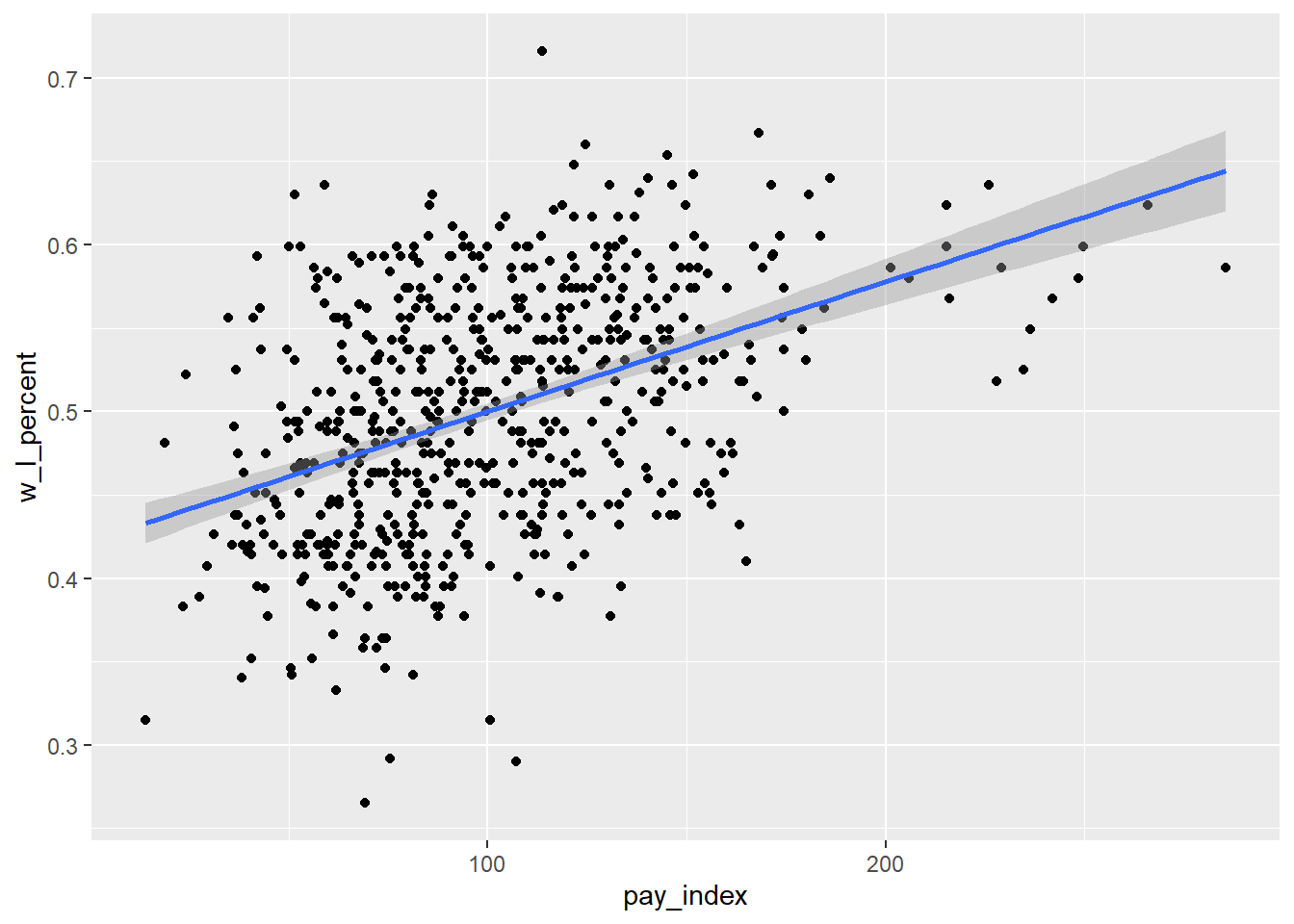
The regression model
We can use the lm() method to create our regression statistics.
# run the regression model, assign the output to an object
model_mlb_pay_wl <- lm(w_l_percent ~ pay_index, data = mlb_pay_wl)

# a glance at the regression results
model_mlb_pay_wl
##
## Call:
## lm(formula = w_l_percent ~ pay_index, data = mlb_pay_wl)
##
## Coefficients:
## (Intercept) pay_index
## 0.4221096 0.0007787The regression equation is the same as an equation for defining a line in Cartesian geometry:
y=b0+b1x1+e
How to read this:
the value of
y(i.e. the point on theyaxis) can be predicted bythe intercept value b0, plus
the coefficient b1 times the value of
x
The distance between that predicted point and the actual point is the error term.
The equation calculated by the lm() function, to create the model model_mlb_pay_wl, is:
^w_l_percent=0.4221+0.0008(pay_index)
This means that any predicted value of y (that is, the y-axis value of any point on the line) is equal to
0.42 +
8^{-4} * the value of x.
If x = 150, then y = 0.42 + (8^{-4} * 150), which is 0.54.
Look back at the line of best fit—if x = 150, the y point on the line is just above the 0.5 mark.
Or another way to think about it: in a 162 game season, a team spending 50% more on payroll than the league average can expect to win 54% (0.54) of their games. This works out to 87 games (162 * 0.54).
We can get more details from the statistical model by using the summary() function, including the P value and the R-squared value:
summary(model_mlb_pay_wl)##
## Call:
## lm(formula = w_l_percent ~ pay_index, data = mlb_pay_wl)
##
## Residuals:
## Min 1Q Median 3Q Max
## -0.215535 -0.048230 0.002686 0.046287 0.205237
##
## Coefficients:
## Estimate Std. Error t value Pr(>|t|)
## (Intercept) 0.42210961 0.00699430 60.35 <0.0000000000000002 ***
## pay_index 0.00077875 0.00006486 12.01 <0.0000000000000002 ***
## ---
## Signif. codes: 0 '***' 0.001 '**' 0.01 '*' 0.05 '.' 0.1 ' ' 1
##
## Residual standard error: 0.06573 on 628 degrees of freedom
## Multiple R-squared: 0.1867, Adjusted R-squared: 0.1854
## F-statistic: 144.2 on 1 and 628 DF, p-value: < 0.00000000000000022Questions
1. Moneyball
(4 marks)
Review the outputs from the model summary above.
Is this model statistically significant? What is the P value?
What is the R-squared value of this model? What does it tell us about the strength of the relationship between these two variables?
If you were managing the budget of a MLB team, would you feel confident telling the shareholders that spending money on star players would turn into success on the field? Explain your answer.
2. Does winning lead to bigger crowds?
(8 marks)
In any sport, successful teams draw bigger crowds. If we were to model this relationship, we would say attendance is the dependent variable, while winning is the independent variable.
Use the data in the “mlb_pay_wl.csv” file to visualize the relationship between team wins (or winning percentage) and attendance.
Use the data in the “mlb_pay_wl.csv” file to create a regression model that evaluates the relationship between team success on the field and attendance. Display the results in your output.
Describe and analyze the coefficients, the R-squared value, and the P value. Can we say that a successful team draw bigger crowds?
3. Data organization in spreadsheets
(4 marks)
Read the following article:
Karl W. Broman and Kara H. Woo, “Data Organization in Spreadsheets”, The American Statistician, Vol 72, Issue 1: Special Issue on Data Science, 2018
- it is available from this link: https://www.tandfonline.com/doi/full/10.1080/00031305.2017.1375989
What are basic principles for using spreadsheets for good data organization?
What are good approaches for handling dates in spreadsheets?