3 An example of a data analytics project
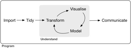
3.1 The data science process
This walkthrough follows the data science process, as described by Hadley Wickham, Mine Çetinkaya-Rundel, and Garrett Grolemund in R for Data Science, 2nd ed..
3.2 New Housing Price Index
This set of scripts creates summary tables and graphs plotting the New Housing Price Index (NHPI) data collected and reported by Statistics Canada.
Our end point will be this chart:
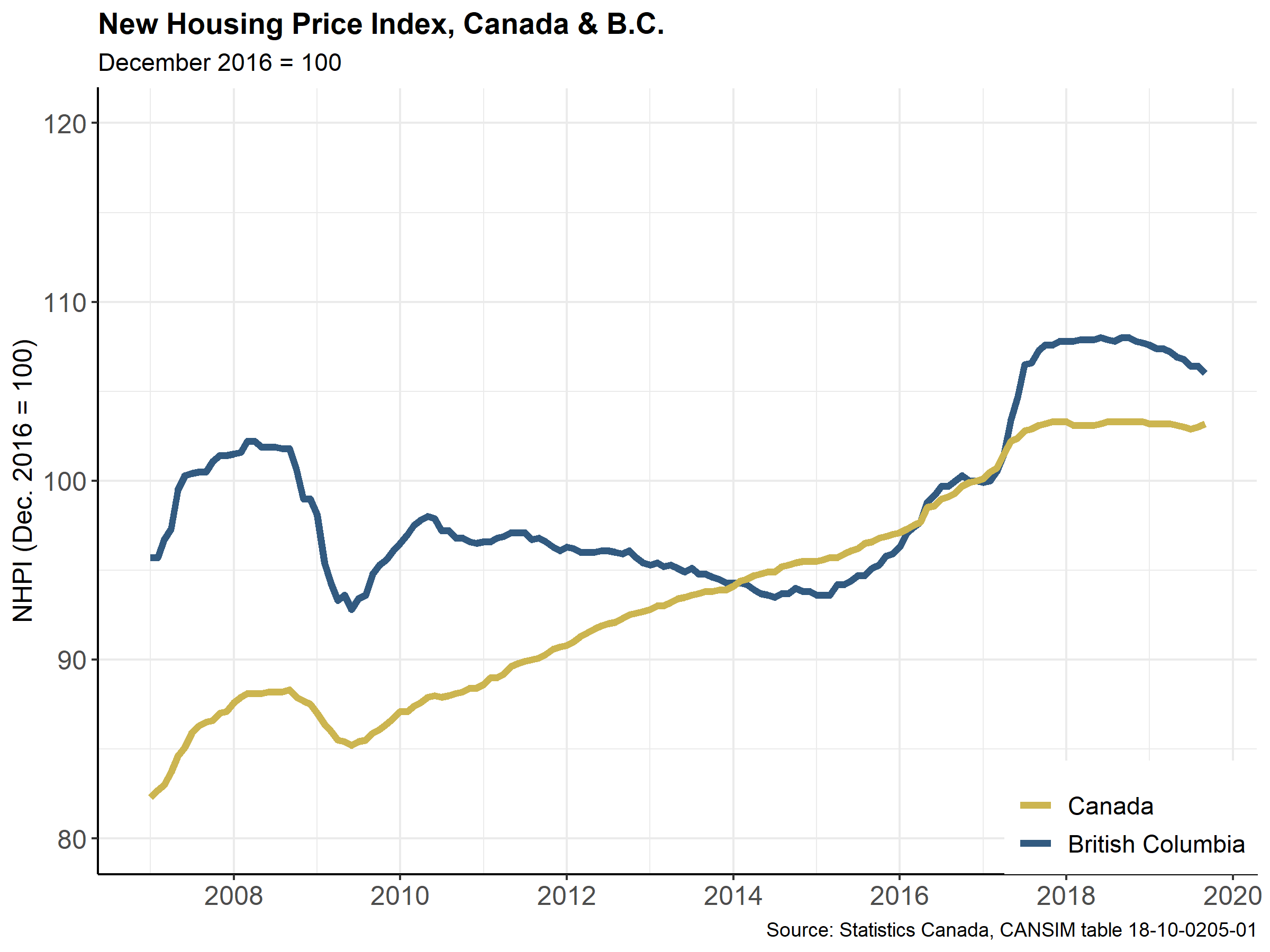
This plot was created in early 2020, when the most recent data available was for the month of November 2019.
3.2.1 Setup
This chunk of R code loads the packages that we will be using.
# tidyverse
library(tidyverse)
library(lubridate)  # date functions
library(scales)     # extending {ggplot2}
library(glue)       # for gluing strings together
#
# utilities
library(cansim)     # data extract
library(janitor)    # for `clean_names()`
library(knitr)      # for publication - includes `kable()` for tables
library(kableExtra) # - format kable tables
library(flextable)  # another table formatting package
First, we have some code for two custom functions that calculate month-over-month and year-over-year statistics. These will be called later in the scripts. Functions give us a shorthand way to do the same thing multiple times.
get_mom_stats <- function(df) {
  df |>
    arrange(ref_date) |>
    mutate(mom_val = lag(value),
           mom_pct = ((value / lag(value, n = 1)) - 1) * 100,
           mom_chg = (value - lag(value, n = 1)))
}


get_yoy_stats <- function(df) {
  df |>
    arrange(ref_date) |>
    mutate(yoy_val = lag(value, n = 12),
           yoy_pct = ((value / lag(value, n = 12)) - 1) * 100,
           yoy_chg = (value - lag(value, n = 12)))
}
We then create a chart theme that will also be called later. This theme will be applied to all of our charts, and ensures that every one of our charts have exactly the same formatting. Like functions, this streamlines our code and helps reduce the chance of error.
For this chart theme, more than 10 lines of code gets reduced to a simple, memorable name: dams_chart_theme.
dams_chart_theme <-
  theme_bw() +
  theme(
    panel.border = element_rect(colour="white"),
    plot.title = element_text(face="bold"),
    legend.position=c(1,0),
    legend.justification=c(1,0),
    legend.title = element_text(size=12),
    legend.text = element_text(size=11),
    axis.line = element_line(colour="black"),
    axis.title = element_text(size=12),
    axis.text = element_text(size=12)
  )
3.3 IMPORT
The first step is to import the data. For this, we will access Statistics Canada’s database CANSIM, using an R package {cansim}. The file has 18 variables and over 56,000 rows (as of February 2020) and growing every month.
data source
Table: 18-10-0205-01 (formerly CANSIM 327-0056) https://www150.statcan.gc.ca/t1/tbl1/en/tv.action?pid=1810020501
Note: “The index base period, for which the New Housing Price Index (NHPI) equals 100, is December 2016.”
This version (updated 2025-11-14) uses the cansim package to pull the data from CANSIM, and assign it to an object named “thedata”.
table_id <- "18-10-0205-01"

thedata <- get_cansim(table_id)
3.4 TIDY
3.4.1 understanding the data
It’s a good practice before starting any data analysis to understand the structure of your data, by interrogating the variables and the values in those variables.
{cansim} (like many other data-focused packages) provides some utility functions that let us quickly understand the data frame. Here we use the function get_cansim_table_overview to generate an overview of the table we downloaded.
# from the {cansim} package
get_cansim_table_overview(table_id)
We can also create some summaries with the names of the variables. One way to do this is with the ls.str() function:
# list the variables in the data
ls.str(thedata)
## Classification Code for New housing price indexes : chr [1:64440] NA NA NA NA NA NA NA NA NA NA NA NA NA NA NA NA NA NA NA NA NA NA NA NA NA NA NA ...
## COORDINATE : chr [1:64440] "1.1" "1.2" "1.3" "2.1" "2.2" "2.3" "3.1" "3.2" "3.3" "4.1" "4.2" "4.3" "5.1" ...
## Date : Date[1:64440], format: "1981-01-01" "1981-01-01" "1981-01-01" "1981-01-01" "1981-01-01" "1981-01-01" ...
## DECIMALS : chr [1:64440] "1" "1" "1" "1" "1" "1" "1" "1" "1" "1" "1" "1" "1" "1" "1" "1" "1" "1" "1" "1" ...
## DGUID : chr [1:64440] "2016A000011124" "2016A000011124" "2016A000011124" "2016A00011" "2016A00011" ...
## GEO : Factor w/ 40 levels "Canada","Atlantic Region",..: 1 1 1 2 2 2 3 3 3 4 ...
## GeoUID : chr [1:64440] "11124" "11124" "11124" "1" "1" "1" "10" "10" "10" "1" "1" "1" "11" "11" "11" ...
## Hierarchy for GEO : chr [1:64440] "1" "1" "1" "1.2" "1.2" "1.2" "1.2.3" "1.2.3" "1.2.3" "1.2.3.4" "1.2.3.4" ...
## Hierarchy for New housing price indexes : chr [1:64440] "1" "1.2" "1.3" "1" "1.2" "1.3" "1" "1.2" "1.3" "1" "1.2" "1.3" "1" "1.2" "1.3" ...
## New housing price indexes : Factor w/ 3 levels "Total (house and land)",..: 1 2 3 1 2 3 1 2 3 1 ...
## REF_DATE : chr [1:64440] "1981-01" "1981-01" "1981-01" "1981-01" "1981-01" "1981-01" "1981-01" "1981-01" ...
## SCALAR_FACTOR : chr [1:64440] "units" "units" "units" "units" "units" "units" "units" "units" "units" "units" ...
## SCALAR_ID : chr [1:64440] "0" "0" "0" "0" "0" "0" "0" "0" "0" "0" "0" "0" "0" "0" "0" "0" "0" "0" "0" "0" ...
## STATUS : chr [1:64440] NA NA "E" ".." ".." ".." ".." ".." ".." NA NA "E" ".." ".." ".." ".." ".." ".." ...
## SYMBOL : chr [1:64440] NA NA NA NA NA NA NA NA NA NA NA NA NA NA NA NA NA NA NA NA NA NA NA NA NA NA NA ...
## TERMINATED : chr [1:64440] NA NA NA NA NA NA NA NA NA NA NA NA NA NA NA NA NA NA NA NA NA NA NA NA NA NA NA ...
## UOM : chr [1:64440] "Index, 201612=100" "Index, 201612=100" "Index, 201612=100" "Index, 201612=100" ...
## UOM_ID : chr [1:64440] "347" "347" "347" "347" "347" "347" "347" "347" "347" "347" "347" "347" "347" ...
## val_norm : num [1:64440] 38.2 36.1 40.6 NA NA NA NA NA NA 36.1 ...
## VALUE : num [1:64440] 38.2 36.1 40.6 NA NA NA NA NA NA 36.1 ...
## VECTOR : chr [1:64440] "v111955442" "v111955443" "v111955444" "v111955445" "v111955446" "v111955447" ...We can explore the individual variables as well—let’s generate a small table counting the instances of the GEO and GeoUID variables:
## # A tibble: 40 × 3
## # Groups:   GEO [40]
##    GEO                                                 GeoUID     n
##    <fct>                                               <chr>  <int>
##  1 Canada                                              11124   1611
##  2 Atlantic Region                                     1       1611
##  3 Newfoundland and Labrador                           10      1611
##  4 St. John's, Newfoundland and Labrador               1       1611
##  5 Prince Edward Island                                11      1611
##  6 Charlottetown, Prince Edward Island                 105     1611
##  7 Nova Scotia                                         12      1611
##  8 Halifax, Nova Scotia                                205     1611
##  9 New Brunswick                                       13      1611
## 10 Saint John, Fredericton, and Moncton, New Brunswick <NA>    1611
## # ℹ 30 more rows
The tail() function shows the last 6 rows of a data table.
tail(thedata)## # A tibble: 6 × 21
## REF_DATE Date GEO DGUID GeoUID New housing price in…¹ VALUE val_norm UOM UOM_ID
## <chr> <date> <fct> <chr> <chr> <fct> <dbl> <dbl> <chr> <chr>
## 1 2025-09 2025-09-01 Vancouver, Br… 2011… 933 Total (house and land) 126. 126. Inde… 347
## 2 2025-09 2025-09-01 Vancouver, Br… 2011… 933 House only 123. 123. Inde… 347
## 3 2025-09 2025-09-01 Vancouver, Br… 2011… 933 Land only 123. 123. Inde… 347
## 4 2025-09 2025-09-01 Victoria, Bri… 2011… 935 Total (house and land) 122. 122. Inde… 347
## 5 2025-09 2025-09-01 Victoria, Bri… 2011… 935 House only 124. 124. Inde… 347
## 6 2025-09 2025-09-01 Victoria, Bri… 2011… 935 Land only 115. 115. Inde… 347
## # ℹ abbreviated name: ¹`New housing price indexes`
## # ℹ 11 more variables: SCALAR_FACTOR <chr>, SCALAR_ID <chr>, VECTOR <chr>, COORDINATE <chr>,
## # STATUS <chr>, SYMBOL <chr>, TERMINATED <chr>, DECIMALS <chr>, `Hierarchy for GEO` <chr>,
## # `Classification Code for New housing price indexes` <chr>,
## # `Hierarchy for New housing price indexes` <chr>Based on this interrogation, we can see that the chart is made up of the following variables:
“REF_DATE”, starting in January 2007
“GEO”, with British Columbia & Canada
“New housing price indexes”, but total (not house and land separately)
3.4.2 cleaning
Cleaning up our data table before we start working is often the next step. In this case, we use the {janitor} package to clean the variable names.
The values in the date field is also problematic—they are stored as character strings. We will clean the values by specifying them as a “date” format.
thedata <- janitor::clean_names(thedata)

thedata <- thedata |>
    mutate(ref_date = ymd(ref_date, truncated = 2))

head(thedata)
## # A tibble: 6 × 21
## ref_date date geo dguid geo_uid new_housing_price_in…¹ value val_norm uom uom_id
## <date> <date> <fct> <chr> <chr> <fct> <dbl> <dbl> <chr> <chr>
## 1 1981-01-01 1981-01-01 Canada 2016… 11124 Total (house and land) 38.2 38.2 Inde… 347
## 2 1981-01-01 1981-01-01 Canada 2016… 11124 House only 36.1 36.1 Inde… 347
## 3 1981-01-01 1981-01-01 Canada 2016… 11124 Land only 40.6 40.6 Inde… 347
## 4 1981-01-01 1981-01-01 Atlantic R… 2016… 1 Total (house and land) NA NA Inde… 347
## 5 1981-01-01 1981-01-01 Atlantic R… 2016… 1 House only NA NA Inde… 347
## 6 1981-01-01 1981-01-01 Atlantic R… 2016… 1 Land only NA NA Inde… 347
## # ℹ abbreviated name: ¹new_housing_price_indexes
## # ℹ 11 more variables: scalar_factor <chr>, scalar_id <chr>, vector <chr>, coordinate <chr>,
## # status <chr>, symbol <chr>, terminated <chr>, decimals <chr>, hierarchy_for_geo <chr>,
## # classification_code_for_new_housing_price_indexes <chr>,
## # hierarchy_for_new_housing_price_indexes <chr>Important Note
The clean_names() function changes the names of the three variables that are shown in the chart:
| Variable: Old Name | New Name |
|---|---|
| REF_DATE | ref_date |
| GEO | geo |
| New housing price indexes | new_housing_price_indexes |
3.4.3 filtering: BC & Canada data
For our chart, we don’t need all the geographic regions—just B.C. and Canada. And for our purposes, we need the total value and want the chart to start in 2007, not 1981.
To do that, we use two functions from the {dplyr} package: filter (to pick the rows we want, based on the values of interest) and select (to pick the columns).
startdate <- as.Date("2007-01-01")
# filter to have BC and Canada
thedata_BC_Can <- thedata |>
  filter(ref_date >= startdate) |>
  filter(geo %in% c("British Columbia", "Canada"),
         new_housing_price_indexes == "Total (house and land)") |>
  select(ref_date, geo, new_housing_price_indexes, value)
head(thedata_BC_Can)
## # A tibble: 6 × 4
## ref_date geo new_housing_price_indexes value
## <date> <fct> <fct> <dbl>
## 1 2007-01-01 Canada Total (house and land) 82.3
## 2 2007-01-01 British Columbia Total (house and land) 95.7
## 3 2007-02-01 Canada Total (house and land) 82.7
## 4 2007-02-01 British Columbia Total (house and land) 95.7
## 5 2007-03-01 Canada Total (house and land) 83
## 6 2007-03-01 British Columbia Total (house and land) 96.73.5 UNDERSTAND
3.5.1 Visualize - tables
One way to understand your data is to create a summary table that is more easily scanned by the human eye.
In this case, we will put the rows as each year, and the columns as the months January through December.
NHPI_table <- thedata_BC_Can |>
  filter(geo == "British Columbia") |>
  mutate(year = year(ref_date),
         month = month(ref_date, label = TRUE)) |>
  select(year, month, value) |>
  pivot_wider(names_from = month, values_from = value) |>
  arrange(desc(year))

# display the table
head(NHPI_table)
## # A tibble: 6 × 13
## year Jan Feb Mar Apr May Jun Jul Aug Sep Oct Nov Dec
## <dbl> <dbl> <dbl> <dbl> <dbl> <dbl> <dbl> <dbl> <dbl> <dbl> <dbl> <dbl> <dbl>
## 1 2025 127. 127. 127. 127. 126. 126. 126 125. 125. NA NA NA
## 2 2024 127. 127. 127. 128. 128. 127 127. 128. 127. 127. 127. 127.
## 3 2023 127. 127. 127. 127. 127 128. 127. 128. 127. 127. 127. 127.
## 4 2022 126. 127 128. 128. 128 128. 129. 129. 129. 128. 128. 128.
## 5 2021 112. 116. 117. 119. 120 120. 120. 121. 122. 123. 124 124.
## 6 2020 106. 106. 106. 106. 106. 106. 107. 108. 110. 112. 112. 112.For the next piece, we will calculate an annual average for each year, and add that column to the table.
This is a good time to say that there are often multiple ways to get to the same result—they are not “right” or “wrong”, just different. Here are three different ways to create a column with the annual average (and there are more):
# how to add annual average
# Julie's genius solution
NHPI_table2 <- NHPI_table |>
  mutate(annual_avg = rowMeans(NHPI_table[-1], na.rm = TRUE))
head(NHPI_table2)
## # A tibble: 6 × 14
## year Jan Feb Mar Apr May Jun Jul Aug Sep Oct Nov Dec annual_avg
## <dbl> <dbl> <dbl> <dbl> <dbl> <dbl> <dbl> <dbl> <dbl> <dbl> <dbl> <dbl> <dbl> <dbl>
## 1 2025 127. 127. 127. 127. 126. 126. 126 125. 125. NA NA NA 126.
## 2 2024 127. 127. 127. 128. 128. 127 127. 128. 127. 127. 127. 127. 127.
## 3 2023 127. 127. 127. 127. 127 128. 127. 128. 127. 127. 127. 127. 127.
## 4 2022 126. 127 128. 128. 128 128. 129. 129. 129. 128. 128. 128. 128.
## 5 2021 112. 116. 117. 119. 120 120. 120. 121. 122. 123. 124 124. 120.
## 6 2020 106. 106. 106. 106. 106. 106. 107. 108. 110. 112. 112. 112. 108.
# Stephanie's genius solution
# starts with the raw data table
NHPI_table3 <- thedata_BC_Can |>
  filter(geo == "British Columbia") |>
  mutate(year = year(ref_date),
         month = month(ref_date, label = TRUE)) |>
  select(year, month, value) |>
  group_by(year) |>
  mutate(annual_avg = mean(value, na.rm = TRUE)) |>
  pivot_wider(names_from = month, values_from = value) |>
  arrange(desc(year))

head(NHPI_table3)
## # A tibble: 6 × 14
## # Groups: year [6]
## year annual_avg Jan Feb Mar Apr May Jun Jul Aug Sep Oct Nov Dec
## <dbl> <dbl> <dbl> <dbl> <dbl> <dbl> <dbl> <dbl> <dbl> <dbl> <dbl> <dbl> <dbl> <dbl>
## 1 2025 126. 127. 127. 127. 127. 126. 126. 126 125. 125. NA NA NA
## 2 2024 127. 127. 127. 127. 128. 128. 127 127. 128. 127. 127. 127. 127.
## 3 2023 127. 127. 127. 127. 127. 127 128. 127. 128. 127. 127. 127. 127.
## 4 2022 128. 126. 127 128. 128. 128 128. 129. 129. 129. 128. 128. 128.
## 5 2021 120. 112. 116. 117. 119. 120 120. 120. 121. 122. 123. 124 124.
## 6 2020 108. 106. 106. 106. 106. 106. 106. 107. 108. 110. 112. 112. 112.This is also a good example of how R is continuously evolving. When this course was first taught in autumn 2019, this is where the section on adding the annual average column ended.
But that ongoing evolution has given us a new {dplyr} function, rowwise(). This function allow us to calculate the average of the specified rows as above. What is required is telling R to treat the functions rowwise(), and then specify what we want using the same sort of functions and syntax that would be required for a column:
NHPI_table4 <- NHPI_table |>
  rowwise() |>
  mutate(annual_avg = mean(c(Jan, Feb, Mar, Apr, May, Jun, Jul, Aug, Sep, Oct, Nov, Dec), na.rm = TRUE))

head(NHPI_table4)
## # A tibble: 6 × 14
## # Rowwise:
## year Jan Feb Mar Apr May Jun Jul Aug Sep Oct Nov Dec annual_avg
## <dbl> <dbl> <dbl> <dbl> <dbl> <dbl> <dbl> <dbl> <dbl> <dbl> <dbl> <dbl> <dbl> <dbl>
## 1 2025 127. 127. 127. 127. 126. 126. 126 125. 125. NA NA NA 126.
## 2 2024 127. 127. 127. 128. 128. 127 127. 128. 127. 127. 127. 127. 127.
## 3 2023 127. 127. 127. 127. 127 128. 127. 128. 127. 127. 127. 127. 127.
## 4 2022 126. 127 128. 128. 128 128. 129. 129. 129. 128. 128. 128. 128.
## 5 2021 112. 116. 117. 119. 120 120. 120. 121. 122. 123. 124 124. 120.
## 6 2020 106. 106. 106. 106. 106. 106. 107. 108. 110. 112. 112. 112. 108.For more information about row-wise operations with {dplyr}, see the following resources:
https://community.rstudio.com/t/dplyr-alternatives-to-rowwise/8071/45
-
https://speakerdeck.com/jennybc/row-oriented-workflows-in-r-with-the-tidyverse
3.6 COMMUNICATE - table
One way we often communicate the data is through a summary table.
The tables above have the data we are interested in, but are not appealing to the eye. Using the {flextable} package, we can apply formatting to the tables above. We can also add things like headers and footnotes.
# print table with {flextable} formatting
NHPI_table4 |>
  flextable() |>
#  add_footer(glue::glue("Source: Statistics Canada, Table {table_id}"))
  add_footer_row(values = glue::glue("Source: Statistics Canada, Table {table_id}"),
                 colwidths = 14)
year |
Jan |
Feb |
Mar |
Apr |
May |
Jun |
Jul |
Aug |
Sep |
Oct |
Nov |
Dec |
annual_avg |
|---|---|---|---|---|---|---|---|---|---|---|---|---|---|
2,025 |
126.7 |
126.8 |
126.9 |
126.8 |
126.3 |
126.1 |
126.0 |
125.2 |
125.4 |
126.24444 |
|||
2,024 |
127.1 |
127.2 |
127.2 |
127.8 |
127.9 |
127.0 |
127.4 |
127.5 |
127.3 |
126.6 |
126.6 |
126.6 |
127.18333 |
2,023 |
127.1 |
126.8 |
126.8 |
126.8 |
127.0 |
127.5 |
127.3 |
127.9 |
127.4 |
127.4 |
127.3 |
127.3 |
127.21667 |
2,022 |
126.2 |
127.0 |
127.7 |
127.9 |
128.0 |
128.1 |
128.7 |
128.7 |
128.7 |
127.8 |
127.7 |
127.6 |
127.84167 |
2,021 |
112.3 |
116.3 |
117.2 |
118.9 |
120.0 |
119.7 |
120.3 |
120.8 |
121.9 |
123.3 |
124.0 |
124.1 |
119.90000 |
2,020 |
105.5 |
105.9 |
106.3 |
106.3 |
106.3 |
106.4 |
107.2 |
108.1 |
110.2 |
111.5 |
111.8 |
111.9 |
108.11667 |
2,019 |
107.6 |
107.4 |
107.4 |
107.2 |
106.9 |
106.8 |
106.4 |
106.4 |
106.0 |
105.8 |
105.3 |
105.7 |
106.57500 |
2,018 |
107.8 |
107.8 |
107.9 |
107.9 |
107.9 |
108.0 |
107.9 |
107.8 |
108.0 |
108.0 |
107.8 |
107.7 |
107.87500 |
2,017 |
99.9 |
100.0 |
100.5 |
101.5 |
103.4 |
104.7 |
106.5 |
106.6 |
107.3 |
107.6 |
107.6 |
107.8 |
104.45000 |
2,016 |
96.3 |
97.1 |
97.4 |
97.7 |
98.8 |
99.2 |
99.7 |
99.7 |
100.0 |
100.3 |
100.0 |
100.0 |
98.85000 |
2,015 |
93.6 |
93.6 |
93.6 |
94.2 |
94.2 |
94.4 |
94.7 |
94.7 |
95.1 |
95.3 |
95.8 |
95.9 |
94.59167 |
2,014 |
94.3 |
94.3 |
94.2 |
93.9 |
93.7 |
93.6 |
93.5 |
93.7 |
93.7 |
94.0 |
93.8 |
93.8 |
93.87500 |
2,013 |
95.3 |
95.4 |
95.2 |
95.3 |
95.1 |
94.9 |
95.1 |
94.8 |
94.8 |
94.6 |
94.5 |
94.3 |
94.94167 |
2,012 |
96.3 |
96.2 |
96.0 |
96.0 |
96.0 |
96.1 |
96.1 |
96.0 |
95.9 |
96.1 |
95.7 |
95.4 |
95.98333 |
2,011 |
96.6 |
96.6 |
96.8 |
96.9 |
97.1 |
97.1 |
97.1 |
96.7 |
96.8 |
96.6 |
96.3 |
96.1 |
96.72500 |
2,010 |
96.5 |
97.0 |
97.5 |
97.8 |
98.0 |
97.9 |
97.2 |
97.2 |
96.8 |
96.8 |
96.6 |
96.5 |
97.15000 |
2,009 |
98.1 |
95.4 |
94.3 |
93.3 |
93.6 |
92.8 |
93.4 |
93.6 |
94.8 |
95.3 |
95.6 |
96.1 |
94.69167 |
2,008 |
101.5 |
101.6 |
102.2 |
102.2 |
101.9 |
101.9 |
101.9 |
101.8 |
101.8 |
100.6 |
99.0 |
99.0 |
101.28333 |
2,007 |
95.7 |
95.7 |
96.7 |
97.3 |
99.5 |
100.3 |
100.4 |
100.5 |
100.5 |
101.1 |
101.4 |
101.4 |
99.20833 |
Source: Statistics Canada, Table 18-10-0205-01 | |||||||||||||
3.6.1 table: monthly summary
This code produces a monthly summary table with the most recent 13 months of B.C. data, which allows for year-over-year comparisons with the same month in the previous year.
The second part of the code then formats the table ready for publication.
# create summary table
tbl_month_BC <-
thedata_BC_Can |>
  filter(geo == "British Columbia") |>
  arrange(ref_date) |>
  # calculate percent change stats
  get_mom_stats() |>
  get_yoy_stats() |>
  # pull year and month
  mutate(year = year(ref_date),
         month = month(ref_date, label = TRUE)) |>
  # select relevant columns, rename as necessary
  select(year, month, value,
         "from previous month" = mom_chg,
         "from same month, previous year" = yoy_chg) |>
  arrange(desc(year), desc(month)) |>
  # just print rows 1 to 13
  slice(1:13)

# print table with {kableExtra} formatting
tbl_month_BC |>
  kable(caption = "NHPI, British Columbia", digits = 1) |>
  kable_styling(bootstrap_options = "striped") |>
  row_spec(0, bold = T, font_size = 14) |>
  row_spec(1, bold = T) |>
add_header_above(c(" " = 3, "index point change" = 2), font_size = 14)| year | month | value | from previous month | from same month, previous year |
|---|---|---|---|---|
| 2025 | Sep | 125.4 | 0.2 | -1.9 |
| 2025 | Aug | 125.2 | -0.8 | -2.3 |
| 2025 | Jul | 126.0 | -0.1 | -1.4 |
| 2025 | Jun | 126.1 | -0.2 | -0.9 |
| 2025 | May | 126.3 | -0.5 | -1.6 |
| 2025 | Apr | 126.8 | -0.1 | -1.0 |
| 2025 | Mar | 126.9 | 0.1 | -0.3 |
| 2025 | Feb | 126.8 | 0.1 | -0.4 |
| 2025 | Jan | 126.7 | 0.1 | -0.4 |
| 2024 | Dec | 126.6 | 0.0 | -0.7 |
| 2024 | Nov | 126.6 | 0.0 | -0.7 |
| 2024 | Oct | 126.6 | -0.7 | -0.8 |
| 2024 | Sep | 127.3 | -0.2 | -0.1 |
3.6.2 text
pull B.C. values for latest month
# filter a B.C.-only data frame

thedata_BC <- thedata_BC_Can |>
  filter(geo == "British Columbia") |>
  arrange(ref_date) |>
  # calculate percent change stats
  get_mom_stats() |>
  get_yoy_stats()

# determine most recent month

latest_ref_date <- max(thedata_BC$ref_date)

this_month <- month(latest_ref_date, label = TRUE)
this_year <- year(latest_ref_date)

this_month_nhpi <- thedata_BC |>
  filter(ref_date == latest_ref_date) |>
  pull(value)
this_month_mom <- thedata_BC |>
  filter(ref_date == latest_ref_date) |>
  pull(mom_chg)
this_month_yoy <- thedata_BC |>
  filter(ref_date == latest_ref_date) |>
  pull(yoy_chg)
Our text:
In Sep 2025, the New Housing Price Index for British Columbia was 125.4. This was a change of 0.2 compared to the previous month, and -1.9 year-over-year.
3.7 UNDERSTAND
3.7.1 Visualize - plot
Making a plot of your data is often a good way to understand what the data can tell us, and helps us think about the story in the data. In this case, we will make a basic plot with just a few lines of code.
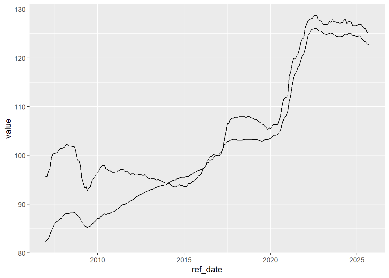
We can make it a little more presentable with some additional formatting
#
# with formatting applied
dataplot <- ggplot(thedata_BC_Can, aes(x=ref_date, y=value, colour=geo)) +
  geom_line(size=1.5)
dataplot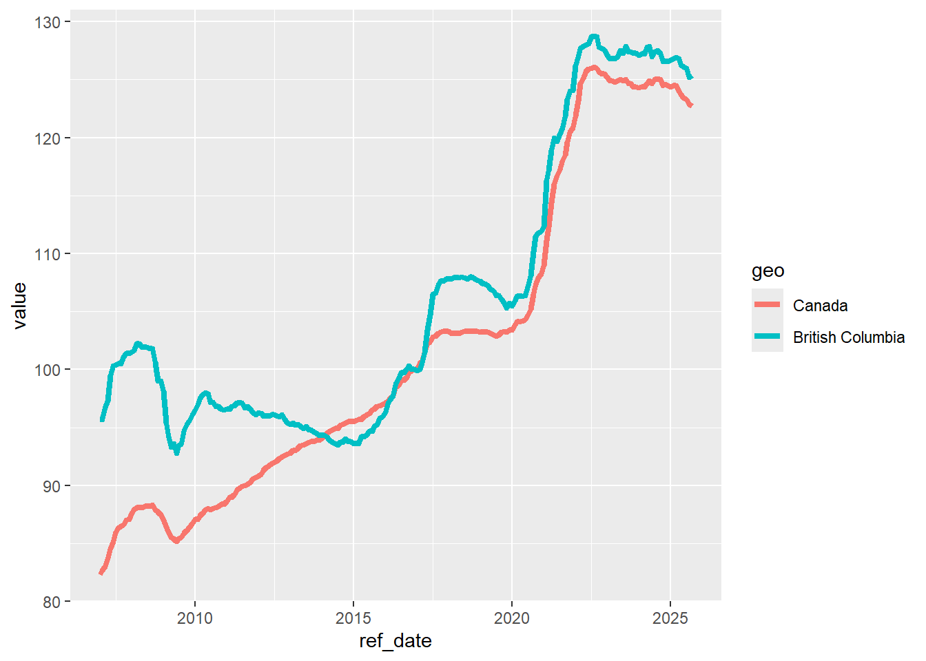
And with even more formatting it’s starting to look like something we could publish.
dataplot2 <- dataplot +
  scale_x_date(date_breaks = "2 years", labels = year) +
  scale_y_continuous(labels = comma, limits = c(80, NA)) +
  scale_colour_manual(name=NULL,
                      breaks=c("Canada", "British Columbia"),
                      labels=c("Canada", "British Columbia"),
                      values=c("#325A80", "#CCB550")) +
  # add the DAMS chart theme elements
  dams_chart_theme
Just a reminder: all of the code below is what’s in the dams_chart_theme—the last line in the code chunk above.
If we were to make more than one copy of the plot, we would have to repeat this every time. And if we made more than one copy of the plot, we would have to make the same change in every place.
By assigning all of this code to the object dams_chart_theme, we can make a change in one place, and it will carry through all of the times we need it.
#  theme_bw() +
#  theme(
#    panel.border = element_rect(colour="white"),
#    plot.title = element_text(face="bold"),
#    legend.position=c(1,0),
#    legend.justification=c(1,0),
#    legend.title = element_text(size=12),
#    legend.text = element_text(size=11),
#    axis.line = element_line(colour="black"),
#    axis.title = element_text(size=12),
#    axis.text = element_text(size=12)
#  )
#
dataplot2 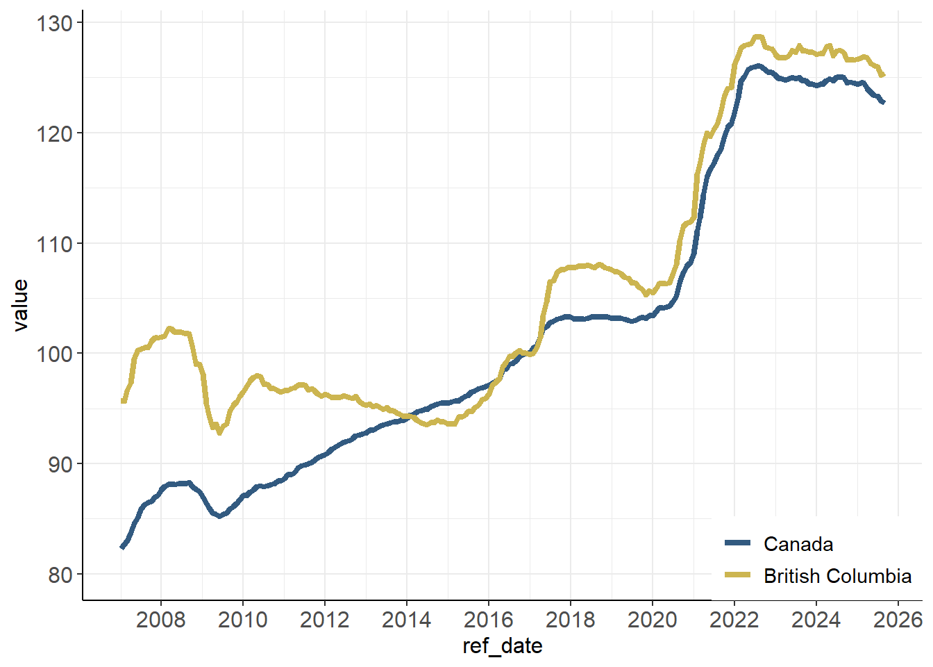
3.8 COMMUNICATE - plot
Let’s finish our formatting…
# experiments with ggplot2's new subtitle and caption options
NHPI_title <- as.character("New Housing Price Index, Canada & B.C.")
NHPI_subtitle <- as.character("December 2016 = 100")
NHPI_caption <- as.character("Source: Statistics Canada, CANSIM table 18-10-0205-01")
# add titles / X-Y axis labels
NHPI_plot <- dataplot2 +
  labs(title = NHPI_title,
       subtitle = NHPI_subtitle,
       caption = NHPI_caption,
       x = NULL, y = "NHPI (Dec. 2016 = 100)")
NHPI_plot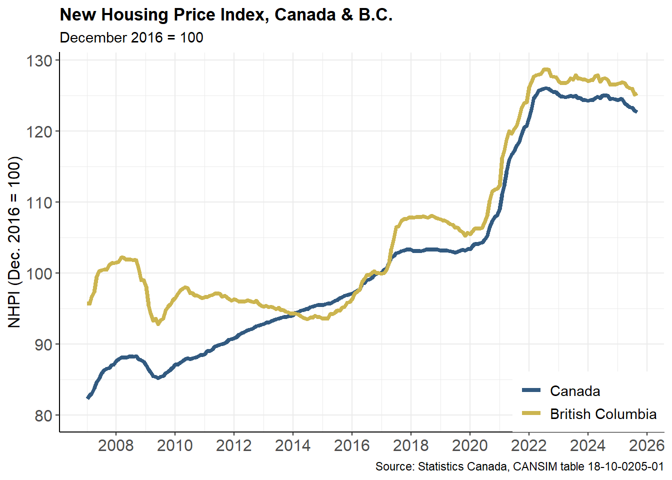
ggsave(filename = "NHPI_plot.jpg", plot = NHPI_plot,
       width = 8, height = 6)
3.9 REPEAT WITH DIFFERENT VALUES
3.9.1 Vancouver house and land version
Now we’ve set up the B.C. comparison to Canada, we can quickly adapt our previous work to look at another region–in this case, a deeper dive into Vancouver, comparing the changes in the “land” and “house” components of the NHPI.
startdate <- as.Date("2007-01-01")

# filter the original data to have Vancouver
thedata_YVR <- thedata |>
  filter(ref_date >= startdate) |>
  filter(geo %in% c("Vancouver, British Columbia"),
         new_housing_price_indexes %in% c("House only", "Land only")) |>
  arrange(desc(ref_date))

thedata_YVR
## # A tibble: 450 × 21
## ref_date date geo dguid geo_uid new_housing_price_in…¹ value val_norm uom uom_id
## <date> <date> <fct> <chr> <chr> <fct> <dbl> <dbl> <chr> <chr>
## 1 2025-09-01 2025-09-01 Vancouver… 2011… 933 House only 123. 123. Inde… 347
## 2 2025-09-01 2025-09-01 Vancouver… 2011… 933 Land only 123. 123. Inde… 347
## 3 2025-08-01 2025-08-01 Vancouver… 2011… 933 House only 122. 122. Inde… 347
## 4 2025-08-01 2025-08-01 Vancouver… 2011… 933 Land only 123. 123. Inde… 347
## 5 2025-07-01 2025-07-01 Vancouver… 2011… 933 House only 123. 123. Inde… 347
## 6 2025-07-01 2025-07-01 Vancouver… 2011… 933 Land only 124. 124. Inde… 347
## 7 2025-06-01 2025-06-01 Vancouver… 2011… 933 House only 123. 123. Inde… 347
## 8 2025-06-01 2025-06-01 Vancouver… 2011… 933 Land only 124. 124. Inde… 347
## 9 2025-05-01 2025-05-01 Vancouver… 2011… 933 House only 125. 125. Inde… 347
## 10 2025-05-01 2025-05-01 Vancouver… 2011… 933 Land only 124. 124. Inde… 347
## # ℹ 440 more rows
## # ℹ abbreviated name: ¹new_housing_price_indexes
## # ℹ 11 more variables: scalar_factor <chr>, scalar_id <chr>, vector <chr>, coordinate <chr>,
## # status <chr>, symbol <chr>, terminated <chr>, decimals <chr>, hierarchy_for_geo <chr>,
## # classification_code_for_new_housing_price_indexes <chr>,
## # hierarchy_for_new_housing_price_indexes <chr>the plot
NHPI_title <- as.character("New Housing Price Index, Vancouver: house and land")
NHPI_subtitle <- as.character("December 2016 = 100")
NHPI_caption <- as.character("Source: Statistics Canada, CANSIM table 18-10-0205-01")

# with formatting applied
NHPI_Vancouver_plot <-
  ggplot(thedata_YVR, aes(x=ref_date, y=value,
                           colour=new_housing_price_indexes)) +
  geom_line(size=1.5) +
  #
  scale_x_date(date_breaks = "2 years", labels = year) +
  scale_y_continuous(labels = comma, limits = c(80, NA)) +
  scale_colour_manual(name=NULL,
                      breaks=c("House only", "Land only"),
                      labels=c("House only", "Land only"),
                      values=c("#325A80", "#CCB550")) +
  dams_chart_theme +
  # set chart titles and labels
  labs(title = NHPI_title,
       subtitle = NHPI_subtitle,
       caption = NHPI_caption,
       x = NULL, y = "NHPI (Dec. 2016 = 100)")

NHPI_Vancouver_plot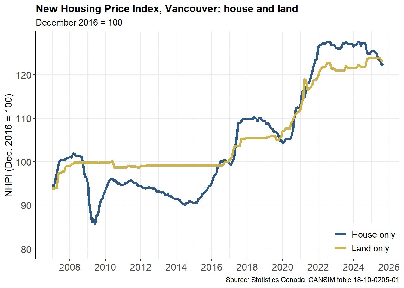
-30-