17 Dates and times
17.2 Objectives
Understand the basics of date and time formats
Understand basic functions in {lubridate} for working with dates
Demonstrate ability to use those functions
17.3 Reading and reference
“Dates and times” in R for Data Science (2nd ed.) by Hadley Wickham, Mine Çetinkaya-Rundel, and Garrett Grolemund
“Strings and Dates” in R Cookbook (2nd ed.)
{lubridate} package reference
17.4 Introduction: Dates and Times
Working with dates and times is an important “tidy” skill, but it also comes into play for the “Understand” phase.
To warm up, try these three seemingly simple questions:
- Does every year have 365 days?
- Does every day have 24 hours?
- Does every minute have 60 seconds?
The answer to all of these is “no”. (See the introduction to the “Dates and Times” chapter of Hadley Wickham, Mine Çetinkaya-Rundel, and Garrett Grolemund R for Data Science (2nd ed.) for explanations.)
To add to the challenge, there are different ways to represent a date. Here’s some ways that March 28, 2020 might be written:
March 28, 2020
2020-03-28
28 Mar 2020
28-3-20
3/28/2020
Saturday, March 28, 2020
Also, keep in mind that a written-out-month is spelled differently in different languages! For example, April in French is “Avril”.
17.4.1 ISO 8601 and R
The ISO 8601 standard is widely recognized as the best way to store dates and times. It removes ambiguity as to which is the day and which is the month (and sometimes the year, if the year is also stored as a two-digit entry). It also sorts in order, with the biggest element (the year) first, followed by the second most important, and so on.
17.5 {lubridate} functions
While dates and times can be complex, the {lubridate} package gives us some tools to work with them.
See https://lubridate.tidyverse.org/reference/index.html
First, today() and now() can be handy. They are based on your computer settings—so whatever time your machine says, now() returns the current time when you run the following code chunk:
now()## [1] "2025-08-27 11:36:55 PDT"You can also specify a time zone:
now(tz = "UTC")## [1] "2025-08-27 18:36:55 UTC"17.6 Parsing
{lubridate} will happily work with numbers and strings, including strings with separators
# a long number
ymd(20200328)
## [1] "2020-03-28"
# a character string, with a two-digit year
ymd("20-03-28")
## [1] "2020-03-28"Parse “10-11-12” using dmy() … what do you get back?
# solution
dmy("10-11-12")
## [1] "2012-11-10"17.6.1 Partials
We sometimes see a partial date. For example, a table showing monthly data might have the dates written as “Jan 2020”, “Feb 2020”, and so on.
{lubridate} parses these by assuming that the date refers to the first day of that month. This then allows us to use the functions below.
my("Jan 2020")## [1] "2020-01-01"17.7 Date
The three functions year(), month(), and day() allow you to extract that component from a ymd value.
Here are three dates:
Here’s how we would get the day from date1:
day(date1)## [1] 2Get the month from date2
# solution

month(date2)
## [1] 2Get the year from date3
year(date3)## [1] 202017.7.0.1 Your turn
What happens when you add the options label and abbr to the function you used to get the day?
- experiment with setting the options to TRUE or FALSE
Solution
# solution
month(date2, label = TRUE, abbr = FALSE)
## [1] February
## 12 Levels: January < February < March < April < May < June < July < August < ... < December17.7.0.2 Your turn
What does wday() do?
Again, experiment with
labelandabbrBonus: what class of variable is
wdayreturning?
Solution
# solution

wday(date1)
## [1] 4
my_wday <- wday(date1, label = TRUE, abbr = FALSE)
my_wday
## [1] Wednesday
## Levels: Sunday < Monday < Tuesday < Wednesday < Thursday < Friday < Saturday
class(my_wday)## [1] "ordered" "factor"## [1] "ordered" "factor"These variables are ordered factors—the days of the week are arranged in a particular order, and using a factor allows that order to be pre-defined.
Another useful function is week(), which returns the week number. More precisely,
week()returns the number of complete seven day periods that have occurred between the date and January 1st, plus one.
We often say that “there are 52 weeks in a year”, but 365 / 7 = 52.1. This means that the last few days of the year are in the 53rd week.
## [1] 1## [1] 5317.8 Time span
There are three classes that we can use:
- durations, which represent an exact number of seconds.
- periods, which represent human units like weeks and months.
- intervals, which represent a starting and ending point.
(from R for Data Science)
The ideas of duration and interval are useful in some contexts, where you want to measure a period of time in seconds. For example, you might be measuring how long it takes an individual on a treadmill to get their heart rate up to 120 beats per minute.
For this exercise, we will keep using our three dates and measure the period between them.
We can subtract two dates:
date2 - date1## Time difference of 423 daysHere’s three different ways of adding a year to a date:
start_date <- ymd("2019-01-01")

start_date + 365
## [1] "2020-01-01"
start_date + dyears(1)## [1] "2020-01-01 06:00:00 UTC"
start_date + years(1)## [1] "2020-01-01"17.9 Working with dates
Read in this extract of a file downloaded from Statistics Canada, which has monthly data showing the British Columbia labour force (both sexes, 15 years and over, unadjusted) from January 2000 to October 2019.
lfs_BC_2000 <- read_csv("data/lfs_BC_2000.csv")
lfs_BC_2000
## # A tibble: 238 × 12
## REF_DATE GEO DGUID Labour force charact…¹ Sex `Age group` Statistics `Data type` UOM
## <chr> <chr> <chr> <chr> <chr> <chr> <chr> <chr> <chr>
## 1 2000-01 British Col… 2016… Labour force Both… 15 years a… Estimate Unadjusted Pers…
## 2 2000-02 British Col… 2016… Labour force Both… 15 years a… Estimate Unadjusted Pers…
## 3 2000-03 British Col… 2016… Labour force Both… 15 years a… Estimate Unadjusted Pers…
## 4 2000-04 British Col… 2016… Labour force Both… 15 years a… Estimate Unadjusted Pers…
## 5 2000-05 British Col… 2016… Labour force Both… 15 years a… Estimate Unadjusted Pers…
## 6 2000-06 British Col… 2016… Labour force Both… 15 years a… Estimate Unadjusted Pers…
## 7 2000-07 British Col… 2016… Labour force Both… 15 years a… Estimate Unadjusted Pers…
## 8 2000-08 British Col… 2016… Labour force Both… 15 years a… Estimate Unadjusted Pers…
## 9 2000-09 British Col… 2016… Labour force Both… 15 years a… Estimate Unadjusted Pers…
## 10 2000-10 British Col… 2016… Labour force Both… 15 years a… Estimate Unadjusted Pers…
## # ℹ 228 more rows
## # ℹ abbreviated name: ¹`Labour force characteristics`
## # ℹ 3 more variables: SCALAR_FACTOR <chr>, VECTOR <chr>, VALUE <dbl>The date is shown in the variable REF_DATE (short for “reference date”); since it’s monthly data, the character representation contains the year and the month, but not the day.
What happens when you mutate REF_DATE into a new variable, using the ymd() function from {lubridate}?
# solution
lfs_BC_2000 |>
  mutate(ref_date_2 = ymd(REF_DATE)) |>
  select(REF_DATE, ref_date_2) |>
  slice(10:15)
## # A tibble: 6 × 2
## REF_DATE ref_date_2
## <chr> <date>
## 1 2000-10 NA
## 2 2000-11 NA
## 3 2000-12 NA
## 4 2001-01 2020-01-01
## 5 2001-02 2020-01-02
## 6 2001-03 2020-01-03Oh no! 94 of the 238 failed to parse—the program was unable to convert them due to ambiguity in the numbers. These show up as “NA” values, such as “2000-01”. {lubridate} is trying to find a year, a month, and a day in this string, and the “00” value doesn’t make sense in this context.
And some of the months that did parse ended up with completely wrong interpretations. The “20” in “2001-01” is interpreted as the year, and the “01”s become the month and day, so it shows up as “2020-01-01”.
Back to the drawing board…
Fortunately, {lubridate} has an argument in the ymd() function that allows us to deal with this. By adding the truncated = 2 argument to the function, the strings are interpreted as missing the last characters. The first day of each month is now added to our new variable.
# solution
lfs_BC_2000 |>
  mutate(ref_date_2 = ymd(REF_DATE, truncated = 2)) |>
  select(REF_DATE, ref_date_2)
## # A tibble: 238 × 2
## REF_DATE ref_date_2
## <chr> <date>
## 1 2000-01 2000-01-01
## 2 2000-02 2000-02-01
## 3 2000-03 2000-03-01
## 4 2000-04 2000-04-01
## 5 2000-05 2000-05-01
## 6 2000-06 2000-06-01
## 7 2000-07 2000-07-01
## 8 2000-08 2000-08-01
## 9 2000-09 2000-09-01
## 10 2000-10 2000-10-01
## # ℹ 228 more rowsAnother approach is to use the ym() function, which yields the same result.
## # A tibble: 238 × 13
## REF_DATE GEO DGUID Labour force charact…¹ Sex `Age group` Statistics `Data type` UOM
## <chr> <chr> <chr> <chr> <chr> <chr> <chr> <chr> <chr>
## 1 2000-01 British Col… 2016… Labour force Both… 15 years a… Estimate Unadjusted Pers…
## 2 2000-02 British Col… 2016… Labour force Both… 15 years a… Estimate Unadjusted Pers…
## 3 2000-03 British Col… 2016… Labour force Both… 15 years a… Estimate Unadjusted Pers…
## 4 2000-04 British Col… 2016… Labour force Both… 15 years a… Estimate Unadjusted Pers…
## 5 2000-05 British Col… 2016… Labour force Both… 15 years a… Estimate Unadjusted Pers…
## 6 2000-06 British Col… 2016… Labour force Both… 15 years a… Estimate Unadjusted Pers…
## 7 2000-07 British Col… 2016… Labour force Both… 15 years a… Estimate Unadjusted Pers…
## 8 2000-08 British Col… 2016… Labour force Both… 15 years a… Estimate Unadjusted Pers…
## 9 2000-09 British Col… 2016… Labour force Both… 15 years a… Estimate Unadjusted Pers…
## 10 2000-10 British Col… 2016… Labour force Both… 15 years a… Estimate Unadjusted Pers…
## # ℹ 228 more rows
## # ℹ abbreviated name: ¹`Labour force characteristics`
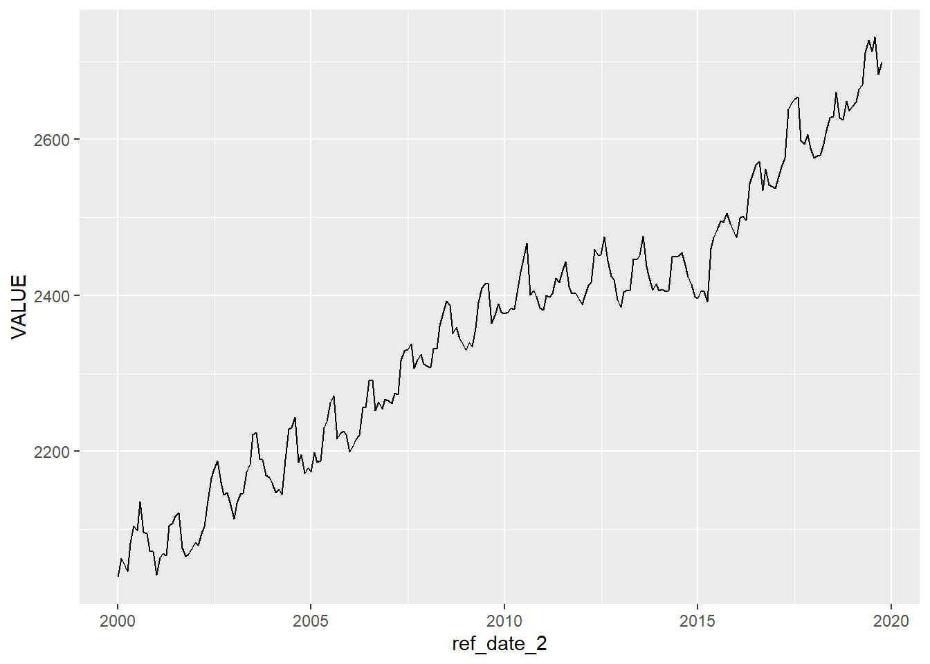
## # ℹ 4 more variables: SCALAR_FACTOR <chr>, VECTOR <chr>, VALUE <dbl>, ref_date_2 <date>With the reference date now turned into a date format, we can create a line plot, and {ggplot2} will make some decisions for us on the format of the labels on the x-axis.
And now we will create a summary table…the annual average of the number of people in the B.C. labour force.
In this code chunk, the variable “ref_date_2” is inside the year() function. This means that the year component of the full date becomes the grouping variable.
## # A tibble: 20 × 2
##    `year(ref_date_2)` annual_average
##                 <dbl>          <dbl>
##  1               2000          2080.
##  2               2001          2082.
##  3               2002          2134.
##  4               2003          2172.
##  5               2004          2186.
##  6               2005          2220.
##  7               2006          2248.
##  8               2007          2304.
##  9               2008          2349.
## 10               2009          2375.
## 11               2010          2405.
## 12               2011          2409.
## 13               2012          2429.
## 14               2013          2425.
## 15               2014          2425.
## 16               2015          2458.
## 17               2016          2532.
## 18               2017          2601.
## 19               2018          2616.
## 20               2019          2689.
Looks like the B.C. labour force is growing!
17.9.0.1 Your turn
Is there any seasonality in the size of the labour force? That is, is there a regular and predictable pattern that repeats each year?
Solution
To calculate the monthly average over the 20 years in our data, we can use the month() function to use the 12 months of the year as our grouping variable.
## # A tibble: 12 × 2
##    `month(ref_date_2)` monthly_average
##                  <dbl>           <dbl>
##  1                   1           2314.
##  2                   2           2324.
##  3                   3           2329.
##  4                   4           2331.
##  5                   5           2369.
##  6                   6           2381.
##  7                   7           2391.
##  8                   8           2402.
##  9                   9           2364.
## 10                  10           2365.
## 11                  11           2342.
## 12                  12           2336.
In this second solution, the mutate() function is used to create a stand-alone variable “ref_month”, which becomes the grouping variable.
The month() function also includes the argument label = TRUE, which adds the abbreviations for the month names.
# solution 2
lfs_BC_2000 |>
  mutate(ref_month = month(ref_date_2, label = TRUE)) |>
  group_by(ref_month) |>
  summarise(monthly_average = mean(VALUE))
## # A tibble: 12 × 2
## ref_month monthly_average
## <ord> <dbl>
## 1 Jan 2314.
## 2 Feb 2324.
## 3 Mar 2329.
## 4 Apr 2331.
## 5 May 2369.
## 6 Jun 2381.
## 7 Jul 2391.
## 8 Aug 2402.
## 9 Sep 2364.
## 10 Oct 2365.
## 11 Nov 2342.
## 12 Dec 2336.Would a simple data visualization (a plot) help you see if there is a pattern?
Of course the answer is “Yes!” Visualization is an important tool in exploratory data analysis. But you knew that already.
(Note that if you haven’t already, you will have to create a separate variable with the month value. As of this writing, {ggplot2} doesn’t allow you to run a function inside the aes().)
lfs_BC_2000 |>
  mutate(ref_month = month(ref_date_2)) |>
  group_by(ref_month) |>
  summarise(monthly_average = mean(VALUE)) |>
  # now plot the resulting summary table
  ggplot(aes(x = ref_month, y = monthly_average)) +
  geom_line()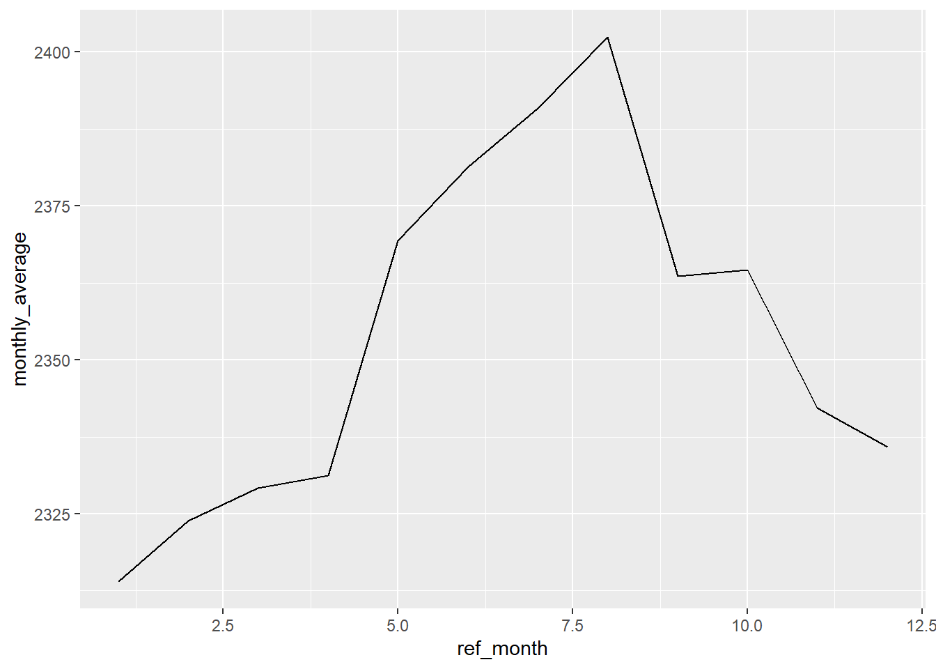
Our plot is a bit off, though, with the x-axis labels showing decimal place months. This is because the “ref_month” variable is a numeric value.
An effective solution is specify the type of scale in the x-axis, using scale_x_discrete().
lfs_BC_2000 |>
  mutate(ref_month = month(ref_date_2)) |>
  group_by(ref_month) |>
  summarise(monthly_average = mean(VALUE)) |>
  ggplot(aes(x = ref_month, y = monthly_average)) +
  geom_line() +
  # add x-axis scale
  scale_x_discrete(limits = month.abb)
Important note: leaving the labels = TRUE will not work with this plot! That’s because it becomes a factor, which can’t be plotted as a line. One solution would be to plot the values using geom_col().
17.10 Date-time
What is the difference between today() and now()?
# solution

today()
## [1] "2025-08-27"
now()## [1] "2025-08-27 11:37:00 PDT"today() is a date, while now() includes the time.
17.10.1 Time zones
You can specify time zones by adding a time zone option to your call. For example, the time zone in the west coast of North America is often represented as “America/Los_Angeles” or “America/Vancouver”.
## [1] "America/Vancouver"What time is it right now? Specify the time zone in the now() function with the argument tzone = or tz =
at the University of Victoria campus—or maybe Vancouver
in St. John’s, Newfoundland
in Lima, Peru
in Seoul, South Korea
in Auckland, New Zealand
and Universal Time Coordinated (the time zone is represented as “UTC”)
# Victoria, British Columbia, Canada
now(tzone = "America/Vancouver")
## [1] "2025-08-27 11:37:01 PDT"
# St. John's, Newfoundland & Labrador, Canada
now(tzone = "America/St_Johns")
## [1] "2025-08-27 16:07:01 NDT"
# Lima, Peru
now(tzone = "America/Lima")
## [1] "2025-08-27 13:37:01 -05"
# Seoul, South Korea
now(tz = "Asia/Seoul")
## [1] "2025-08-28 03:37:01 KST"
# Auckland, New Zealand
now(tz = "Pacific/Auckland")
## [1] "2025-08-28 06:37:01 NZST"
# Universal Time Coordinated (UTC)
now(tz = "UTC")
## [1] "2025-08-27 18:37:01 UTC"Some things to notice:
St. John’s is 30 minutes off-set from the other time zones
Lima doesn’t appear with a named “time” unlike the others, but is -05 hours relative to UTC
For those of us in the western hemisphere, it’s almost always tomorrow in South Korea and New Zealand!
You can use the function OlsonNames() (from base R) to print a list of all 597 time zones around the world!
# solution -- beware the length!
head(OlsonNames())
## [1] "Africa/Abidjan" "Africa/Accra" "Africa/Addis_Ababa" "Africa/Algiers"
## [5] "Africa/Asmara" "Africa/Asmera"(Note: wrapping a function call with an assignment both runs the assignment and prints the object!)
(x1 <- ymd_hms("2015-06-01 12:00:00", tz = "America/New_York"))## [1] "2015-06-01 12:00:00 EDT"
(x2 <- ymd_hms("2015-06-01 18:00:00", tz = "Europe/Copenhagen"))## [1] "2015-06-01 18:00:00 CEST"
(x3 <- ymd_hms("2015-06-02 04:00:00", tz = "Pacific/Auckland"))## [1] "2015-06-02 04:00:00 NZST"Subtract date-time from each other
#
x2 - x3
## Time difference of 0 secs17.11 Lead and lag
df_dates <- tribble(~event, ~event_date,
        "event_1", "2015-01-15",
        "event_2", "2020-02-29",
        "event_3", "2020-04-15"
        )

df_dates <- df_dates |>
  mutate(event_date = ymd(event_date))

df_dates
## # A tibble: 3 × 2
## event event_date
## <chr> <date>
## 1 event_1 2015-01-15
## 2 event_2 2020-02-29
## 3 event_3 2020-04-15
df_summary <- df_dates |>
  # create a new variable with the lag from the previous record
  mutate(lag_date = lag(event_date)) |>
  # calculate the different between the two dates
  mutate(days_between = event_date - lag_date)

df_summary
## # A tibble: 3 × 4
## event event_date lag_date days_between
## <chr> <date> <date> <drtn>
## 1 event_1 2015-01-15 NA NA days
## 2 event_2 2020-02-29 2015-01-15 1871 days
## 3 event_3 2020-04-15 2020-02-29 46 daysTo calculate the number of years (instead of days), we the need to convert “days_between” from Duration to integer before dividing by 365.25.
df_summary |>
  mutate(years_between = as.integer(days_between)/365.25)
## # A tibble: 3 × 5
## event event_date lag_date days_between years_between
## <chr> <date> <date> <drtn> <dbl>
## 1 event_1 2015-01-15 NA NA days NA
## 2 event_2 2020-02-29 2015-01-15 1871 days 5.12
## 3 event_3 2020-04-15 2020-02-29 46 days 0.126## # A tibble: 1 × 1
## avg_days_between_events
## <drtn>
## 1 958.5 days17.12 Additional references
17.12.1 Other units of time
Financial calendars
- 4-4-5 calendar: each quarter is divided into three “months”, of 4 or 5 weeks length
17.12.2 More {lubridate}
Working with dates and time in R using the lubridate package, University of Virginia Library Research Data Services + Sciences
17.12.3 Other R packages
{clock}: a brand-new package for working with date-times
- Comprehensive Date-Time Handling for R. “lubridate will never go away, and is not being deprecated or superseded. As of now, we consider clock to be an alternative to lubridate.”
17.12.4 Time zones
Randy Au, “Hidden treasure in the timezone database: It’s lie a storybook”, 2022-03-22
-30-