7 Tidy data
7.1 Objectives
Restructure data tabulations with
pivot_wider()andpivot_longer()using
ungroup()to remove the effect of agroup_by()function
7.2 Reading
Hadley Wickham, Mine Çetinkaya-Rundel, and Garrett Grolemund, R for Data Science, 2nd ed.
Karl Broman & Kara Woo, “Data Organization in Spreadsheets”(Broman and Woo 2017)
Julie Lowndes and Allison Horst, “Tidy Data for Efficiency, Reproducibility, and Collaboration”)(Lowndes and Horst 2020)
7.4 Transform Data 3: changing the layout
7.4.1 Tidy and untidy data
In the dataframes we have used so far, the data is in a format that adheres to the rules of tidy data, where
- each column is a variable
- each row is an observation
- each value has its own cell
This is called a “long” data format. But, we notice that each column represents a different variable. In the “longest” data format there would only be three columns, one for the id variable, one for the observed variable, and one for the observed value (of that variable). This data format is quite unsightly and difficult to work with, so you will rarely see it in use.
Alternatively, in a “wide” data format we see modifications to rule 1, where each column no longer represents a single variable. Instead, columns can represent different levels/values of a variable. For instance, in some data you encounter the researchers may have chosen for every survey date to be a different column.
These may sound like dramatically different data layouts, but there are some tools that make transitions between these layouts much simpler than you might think! The gif below shows how these two formats relate to each other, and gives you an idea of how we can use R to shift from one format to the other.
(From the Data Carpentry lesson R for Social Scientists, “Data Wrangling with dplyr and tidyr”—this lesson provides a different example of using {tidyr} to reshape your data.)
The image below shows the relationship between the two versions of the same data:[@AdenBuie_tidyanimated]
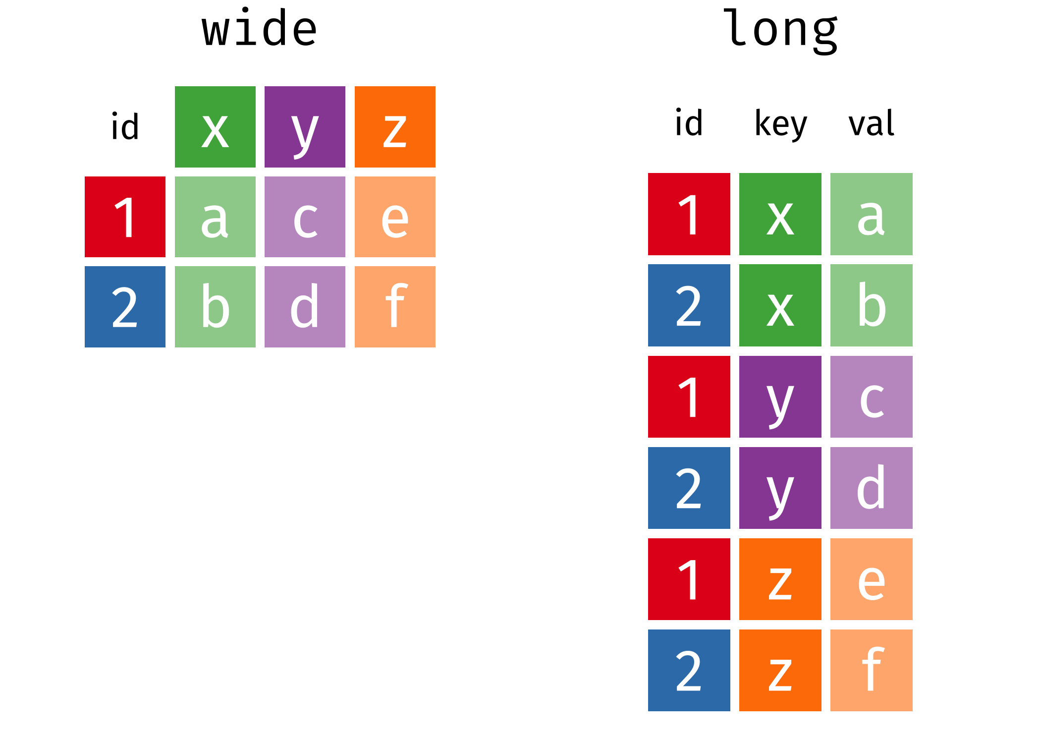
The “wide” form doesn’t adhere to the rules of tidy data, since each row has multiple observations.
Untidy data most often look like this: * Column headers are values, not variable names. * Multiple variables are stored in one column. * Variables are stored in both rows and columns. * Multiple types of observational units are stored in the same table. * A single observational unit is stored in multiple tables.
(Source: John Spencer, “Tidy Data and How to Get It”)
7.4.2 An example
Let’s create a pivot table crosstab using the penguin data in the {palmerpenguins} data package.
First, a look at the source table.
penguins## # A tibble: 344 × 8
## species island bill_length_mm bill_depth_mm flipper_length_mm body_mass_g sex year
## <fct> <fct> <dbl> <dbl> <int> <int> <fct> <int>
## 1 Adelie Torgersen 39.1 18.7 181 3750 male 2007
## 2 Adelie Torgersen 39.5 17.4 186 3800 female 2007
## 3 Adelie Torgersen 40.3 18 195 3250 female 2007
## 4 Adelie Torgersen NA NA NA NA <NA> 2007
## 5 Adelie Torgersen 36.7 19.3 193 3450 female 2007
## 6 Adelie Torgersen 39.3 20.6 190 3650 male 2007
## 7 Adelie Torgersen 38.9 17.8 181 3625 female 2007
## 8 Adelie Torgersen 39.2 19.6 195 4675 male 2007
## 9 Adelie Torgersen 34.1 18.1 193 3475 <NA> 2007
## 10 Adelie Torgersen 42 20.2 190 4250 <NA> 2007
## # ℹ 334 more rowsUse group_by and summarise to create a summary table of the average bird weight by species. Note that we have to use na.rm = TRUE because of the presence of NA values in the variable body_mass_g.
## # A tibble: 3 × 2
##   species   mass_mean
##   <fct>         <dbl>
## 1 Adelie        3701.
## 2 Chinstrap     3733.
## 3 Gentoo        5076.
Now if we do the same with species and island, we end up with a much longer table. Since we are going to restructure this table, it will be assigned to a new object penguin_species_by_island.
penguin_species_by_island <- penguins |>
  group_by(species, island) |>
  summarise(mass_mean = mean(body_mass_g, na.rm = TRUE))

penguin_species_by_island
## # A tibble: 5 × 3
## # Groups: species [3]
## species island mass_mean
## <fct> <fct> <dbl>
## 1 Adelie Biscoe 3710.
## 2 Adelie Dream 3688.
## 3 Adelie Torgersen 3706.
## 4 Chinstrap Dream 3733.
## 5 Gentoo Biscoe 5076.While this long tabular structure is useful for coding, it’s harder for you and I to compare across both the “species” and “island” dimensions. This is a situation where a wide structure is desirable.
7.4.3 pivot_wider()
Let’s take the penguin_species_by_island table and arrange it so that there is a separate column (variable) for each island. Instead of a single “island” column, there will be multiple columns, one for each island, and with the average weight of the birds of each species on each.
You will note that this is NOT a tidy format! But is it one that is human-readable, and is often how data tables are published in reports.
# pivot table (wide)

penguin_species_by_island_pivot <- penguin_species_by_island |>
  pivot_wider(names_from = island, values_from = mass_mean)

penguin_species_by_island_pivot
## # A tibble: 3 × 4
## # Groups: species [3]
## species Biscoe Dream Torgersen
## <fct> <dbl> <dbl> <dbl>
## 1 Adelie 3710. 3688. 3706.
## 2 Chinstrap NA 3733. NA
## 3 Gentoo 5076. NA NANote that there are “NA” values introduced into the table. Chinstrap penguins were only recorded on Dream Island, and Gentoo penguins were only on Biscoe Island…NA values appear in the columns where there were no birds of that species row.
7.4.4 pivot_longer()
Now we will pivot the new table back to the original structure. Note that the names of the new variables “island” and “mean_mass” need to be inside quotation marks!
# and back to longer...

penguin_species_by_island_unpivot <- penguin_species_by_island_pivot |>
  pivot_longer(-species, names_to = "island", values_to = "mean_mass")

penguin_species_by_island_unpivot
## # A tibble: 9 × 3
## # Groups: species [3]
## species island mean_mass
## <fct> <chr> <dbl>
## 1 Adelie Biscoe 3710.
## 2 Adelie Dream 3688.
## 3 Adelie Torgersen 3706.
## 4 Chinstrap Biscoe NA
## 5 Chinstrap Dream 3733.
## 6 Chinstrap Torgersen NA
## 7 Gentoo Biscoe 5076.
## 8 Gentoo Dream NA
## 9 Gentoo Torgersen NAWhat do you notice about the structure of the unpivoted table?
The creation of the wider table introduced “NA” values where there was not an “island” category to match the “species” of penguin. In our new long table, those “NA” values have been retained.
7.4.5 spread() and gather()
Note that pivot_wider() and pivot_longer() are relatively new functions, introduced in 2019.
The older {tidyr} functions that do the same thing: spread() and gather(). You may find older articles that use these functions…but the new ones are much better!
For example, spread() to replicate the pivot_wider() function:
penguin_species_by_island |>
  spread(key = island, value = mass_mean)
## # A tibble: 3 × 4
## # Groups: species [3]
## species Biscoe Dream Torgersen
## <fct> <dbl> <dbl> <dbl>
## 1 Adelie 3710. 3688. 3706.
## 2 Chinstrap NA 3733. NA
## 3 Gentoo 5076. NA NA7.5 Exercises
7.5.1 Canadian election results
This table shows the national-level results of the Federal Election held in Canada on October 10, 2019. This is structure as the table was published by Elections Canada.
## # A tibble: 12 × 3
##    party          category  number
##    <chr>          <chr>      <dbl>
##  1 Liberal        seats        157
##  2 Liberal        votes    5915950
##  3 Conservative   seats        121
##  4 Conservative   votes    6155662
##  5 Bloc Québécois seats         32
##  6 Bloc Québécois votes    1376135
##  7 New Democratic seats         24
##  8 New Democratic votes    2849214
##  9 Green          seats          3
## 10 Green          votes    1162361
## 11 Independent    seats          1
## 12 Independent    votes      75836
1. What tidy data principles does this table violate?
2. Tidy this table’s structure
Solution
1. What tidy data principles does this table violate?
It violiates Principles #1 & #2
- There are two variables (seats and votes) combined into one column
- There are two rows (seats and rows) for each observation (in this case, party)
Sometimes untidy data can be too long!
2. Tidy this table’s structure
To tidy the table, we need to pivot_wider()
# solution

CDN_elec_2019 |>
  pivot_wider(names_from = category, values_from = number)
## # A tibble: 6 × 3
## party seats votes
## <chr> <dbl> <dbl>
## 1 Liberal 157 5915950
## 2 Conservative 121 6155662
## 3 Bloc Québécois 32 1376135
## 4 New Democratic 24 2849214
## 5 Green 3 1162361
## 6 Independent 1 758367.5.2 gapminder
When we publish our tables, we might want a structure that violates the tidy principles—sometimes an untidy table is better for human consumption. The {gapminder} data, in its raw form, is tidy. For this exercise, create a table that shows:
- GDP per capita for
- the countries Canada, United States, and Mexico are the columns, and
- the years after 1980 are the rows
Solution
# solution #1
gapminder |>
  filter(country %in% c("Canada", "United States", "Mexico") &
           year > 1980) |>
  select(country, year, gdpPercap) |>
  pivot_wider(names_from = country, values_from = gdpPercap)
## # A tibble: 6 × 4
## year Canada Mexico `United States`
## <int> <dbl> <dbl> <dbl>
## 1 1982 22899. 9611. 25010.
## 2 1987 26627. 8688. 29884.
## 3 1992 26343. 9472. 32004.
## 4 1997 28955. 9767. 35767.
## 5 2002 33329. 10742. 39097.
## 6 2007 36319. 11978. 42952.
# a similar solution that uses "or" for the countries
# and two separate filter statements
gapminder |>
  filter(country == "Canada" | country == "United States" | country == "Mexico") |>
  filter(year > 1980) |>
  select(country, year, gdpPercap) |>
  pivot_wider(names_from = country, values_from = gdpPercap)
## # A tibble: 6 × 4
## year Canada Mexico `United States`
## <int> <dbl> <dbl> <dbl>
## 1 1982 22899. 9611. 25010.
## 2 1987 26627. 8688. 29884.
## 3 1992 26343. 9472. 32004.
## 4 1997 28955. 9767. 35767.
## 5 2002 33329. 10742. 39097.
## 6 2007 36319. 11978. 42952.Here’s an alternative approach that avoids the use of the select() function.
Note that by adding year to the pivot_wider() all the variables in the final table are explicitly named in the function, and all the other variables in the source table are dropped.
gapminder |>
  filter(country == "Canada" | country == "United States" | country == "Mexico") |>
  filter(year > 1980) |>
  pivot_wider(id_cols = year,
              names_from = "country",
              values_from = "gdpPercap")
## # A tibble: 6 × 4
## year Canada Mexico `United States`
## <int> <dbl> <dbl> <dbl>
## 1 1982 22899. 9611. 25010.
## 2 1987 26627. 8688. 29884.
## 3 1992 26343. 9472. 32004.
## 4 1997 28955. 9767. 35767.
## 5 2002 33329. 10742. 39097.
## 6 2007 36319. 11978. 42952.In this version, the three variables continent, lifeExp, and pop are dropped with the minus sign—the remaining variables are then reshaped.
gapminder |>
  filter(country %in% c("Canada", "United States", "Mexico")) |>
  filter(year > 1980) |>
  pivot_wider(id_cols = c(-continent, -lifeExp, -pop),
              names_from = "country",
              values_from = "gdpPercap")
## # A tibble: 6 × 4
## year Canada Mexico `United States`
## <int> <dbl> <dbl> <dbl>
## 1 1982 22899. 9611. 25010.
## 2 1987 26627. 8688. 29884.
## 3 1992 26343. 9472. 32004.
## 4 1997 28955. 9767. 35767.
## 5 2002 33329. 10742. 39097.
## 6 2007 36319. 11978. 42952.It’s also possible to have multiple columns selected using the id_cols = argument:
# Three countries from three different continents
gapminder |>
  filter(country %in% c("Canada", "China", "Croatia")) |>
  filter(year > 1980) |>
  pivot_wider(id_cols = c(country, continent),
              names_from = "year",
              values_from = "gdpPercap")
## # A tibble: 3 × 8
## country continent `1982` `1987` `1992` `1997` `2002` `2007`
## <fct> <fct> <dbl> <dbl> <dbl> <dbl> <dbl> <dbl>
## 1 Canada Americas 22899. 26627. 26343. 28955. 33329. 36319.
## 2 China Asia 962. 1379. 1656. 2289. 3119. 4959.
## 3 Croatia Europe 13222. 13823. 8448. 9876. 11628. 14619.In the examples above, the steps from the source gapminder dataframe to the three country table are completed in a single pipe. But what if we want to create two separate tables with the same three countries, but one with GDP per capita as the values and the second with life expectancy?
To do this, we create an intermediate object that filters for the year range and the countries we are interested in.
After that object is created, we can use it to first select for the variables we want, and then to pivot.
# create intermediate dataframe "gapminder1"
gapminder1 <- gapminder |>
  filter(year > 1980) |>
  filter(country == "Canada" | country == "Mexico" | country == "Brazil")

# now using the `id_cols = year`, pull the values from gdpPercap
gapminder1 |>
  pivot_wider(id_cols = year,
              names_from = country,
              values_from = gdpPercap)
## # A tibble: 6 × 4
## year Brazil Canada Mexico
## <int> <dbl> <dbl> <dbl>
## 1 1982 7031. 22899. 9611.
## 2 1987 7807. 26627. 8688.
## 3 1992 6950. 26343. 9472.
## 4 1997 7958. 28955. 9767.
## 5 2002 8131. 33329. 10742.
## 6 2007 9066. 36319. 11978.
# and now a 2nd version with life expectancy, pull the values from lifeExp
gapminder1 |>
  pivot_wider(id_cols = year,
              names_from = country,
              values_from = lifeExp)
## # A tibble: 6 × 4
## year Brazil Canada Mexico
## <int> <dbl> <dbl> <dbl>
## 1 1982 63.3 75.8 67.4
## 2 1987 65.2 76.9 69.5
## 3 1992 67.1 78.0 71.5
## 4 1997 69.4 78.6 73.7
## 5 2002 71.0 79.8 74.9
## 6 2007 72.4 80.7 76.27.6 Further reading
More about tidy data:
“Tidy Data for Efficiency, Reproducibility, and Collaboration”)
Data Organization in Spreadsheets for Social Scientists: Formatting problems – this DataCarpentry lesson has some good visuals that may help with understanding “names_from” and “names_to” etc.
Reshaping Your Data with tidyr, UC Business Analytics R Programming Guide
- this article uses the old {tidyr}
gather()andspread()functions instead ofpivot_longer()andpivot_wider(), but it’s got some good material on how to think about how and why data needs to be reshaped.
Julia Lowndes and Allison Horst, Tidy data for efficiency, reproducibility, and collaboration
- in google slide version: “Make friends with tidy data”
Hadley Wickham. “Tidy data”, The Journal of Statistical Software, vol. 59, 2014.
Data organization with spreadsheets – from Data Management Workshop à la CHONe