18 Strings
18.1 Objectives
Understand the basics of regular expressions (regexps)
Understand basic functions in {stringr} for working with strings
Demonstrate ability to use those functions
18.2 Readings and reference
“Strings” in R for Data Science (2nd ed.) by Hadley Wickham, Mine Çetinkaya-Rundel, and Garrett Grolemund
“Strings and Dates” in R Cookbook (2nd ed.)
Regular expressions
18.4 Setup
This chunk of R code loads the packages that we will be using.
Strings are characters, numbers, etc. that are enclosed inside quotation marks. A character vector is made up of multiple strings.
string1 <- "This is my 1st string!"

string1
## [1] "This is my 1st string!"18.5 Regular expressions
regular expressions becomes shortened to “regex”
regexps are a concise language for describing patterns in strings
They are powerful ways to filter and manipulate strings based on those patterns. But they have a certain reputation:
Some people, when confronted with a problem, think “I know, I’ll use regular expressions.” Now they have two problems. – Jamie Zawinski
18.5.1 regex matching functions
Here are some basic matching functions:
Note: the square brackets enclose the regex to identify a single character. In the examples below, with three sets of square brackets, “[a][b][c]” contains three separate character positions, whereas “[abc]” is identifying a single character.
| character | what it does |
|---|---|
| “abc” | matches “abc” |
| “[a][b][c]” | matches “abc” |
| “[abc]” | matches “a”, “b”, or “c” |
| “[^abc]” | matches anything except “a”, “b”, or “c” |
| “^” | match start of string |
| “$” | match end of string |
The {stringr} function str_view() shows where in our string the pattern appears. First we create an object “fruit_list” with three strings in it, then find two different patterns.
## [1] │ <a>pple
# which words have an "ea" combination?
str_view(fruit_list, "ea")
## [3] │ p<ea>rfrequency of match
| character | what it does |
|---|---|
| “?” | 0 or 1 |
| “+” | 1 or more |
| “*” | 0 or more |
The question mark is useful for words with various spellings—the British and American variations of words like “colour” and “neighbour”.
| character | what it does |
|---|---|
| “{n}” | exactly n times |
| “{n,}” | n or more |
| “{n,m}” | between n and m times |
# which words have a double "p"?

str_view(fruit_list, "p{2}")
## [1] │ a<pp>le18.6 Special characters
quotes
To find single and double quotes in our string, they need to be “escaped” with a backslash \.
double_quote <- "\"" # or '"'
single_quote <- '\'' # or "'"

double_quote
## [1] "\""
single_quote## [1] "'"- to see a representation of the string as it will print, use the function
writeLines()
writeLines(double_quote)## "
string2 <- 'The 2nd string has a "quote" so it is inside single quotes'

string2
## [1] "The 2nd string has a \"quote\" so it is inside single quotes"
writeLines(string2)## The 2nd string has a "quote" so it is inside single quotesother special characters
These also need to be escaped:
| character | what it is |
|---|---|
| “\” | backslash |
| “ | any digit |
| “” | newline (line break) |
| “” | any whitespace (space, tab, newline) |
| “ | tab |
| “*” | asterisk |
| “..” | unicode characters* |
See the help function for ?'"'
interrobang <- "\u2048"
interrobang
## [1] "⁈"To make a shruggie, you need to escape the backslash.
shruggie <- "¯\\_(ツ)_/¯"
shruggie
## [1] "¯\\_(ツ)_/¯"
shruggie <- glue::glue("¯\\", "_(ツ)_", "/¯")
shruggie
## ¯\_(ツ)_/¯18.7 Basic functions

Some {stringr} functions
| function | purpose |
|---|---|
| str_length(x) | the number of characters in x
|
| str_c() | concatenates a list of strings |
| str_sub(x, start = , end = ) | returns characters of x
|
| str_detect(string, pattern) | TRUE/FALSE if there is a pattern match |
| str_replace(string, pattern, newtext) | replace |
| str_remove(string, pattern) | removes the first instance of pattern
|
| str_remove_all (string, pattern) | removes all instances of pattern
|
| str_trim (string) | removes whitespace at the beginning and end |
The full list of {stringr} functions can be found at https://stringr.tidyverse.org/reference/index.html
musician_first <- c("Sly", "Billie", "Thelonious", "Maroon", "Willie", "Led")
musician_first
## [1] "Sly" "Billie" "Thelonious" "Maroon" "Willie" "Led"
str_length(musician_first) ## [1] 3 6 10 6 6 3use str_c to collapse list into one string
str_c(musician_first, collapse = ", ")## [1] "Sly, Billie, Thelonious, Maroon, Willie, Led"18.8 Combining strings
Use str_c to join two character vectors, separated by a space.
musician_last <- c("Stone", "Ellish", "Monk", "5", "Nelson", "Zeppelin")

str_c(musician_first, musician_last, sep = " ")
## [1] "Sly Stone" "Billie Ellish" "Thelonious Monk" "Maroon 5" "Willie Nelson"
## [6] "Led Zeppelin"18.8.0.1 Your turn
Now join musician_first to musician_last (the other way around!), separated by an apostrophe and a space.
Solution
#solution
str_c(musician_last, musician_first, sep = ", ")
## [1] "Stone, Sly" "Ellish, Billie" "Monk, Thelonious" "5, Maroon" "Nelson, Willie"
## [6] "Zeppelin, Led"18.9 Pattern matching
18.9.0.1 Your turn
Are there any vowels in the string musician_first?
Use str_detect() to find them, and count them with str_count().
Solution
# solution
str_detect(musician_first, "[aeiou]")
## [1] FALSE TRUE TRUE TRUE TRUE TRUE
str_count(musician_first, "[aeiou]")## [1] 0 3 5 3 3 118.9.0.2 Your turn
Are there any digits in musician_last?
Solution
Don’t forget that you need to escape any backslashes you use!
# solution
str_detect(musician_last, "\\d")
## [1] FALSE FALSE FALSE TRUE FALSE FALSEWe can extract chunks of text by their location using the following function: str_sub(musician_first, start, end).
# solution
str_sub(musician_first, 1, 2)
## [1] "Sl" "Bi" "Th" "Ma" "Wi" "Le"str_locate() finds the first position of the pattern:
# look for pairs of vowels
str_locate(musician_first, "[aeiou][aeiou]")
## start end
## [1,] NA NA
## [2,] 5 6
## [3,] 7 8
## [4,] 4 5
## [5,] 5 6
## [6,] NA NA
# look for a specific match ...
str_locate(musician_first, "oo")
## start end
## [1,] NA NA
## [2,] NA NA
## [3,] NA NA
## [4,] 4 5
## [5,] NA NA
## [6,] NA NAExtract the first case of a vowel:
str_extract(musician_first, "[aeiou]")## [1] NA "i" "e" "a" "i" "e"Extract the pairs of vowels:
# solution
str_extract(musician_first, "[aeiou][aeiou]")
## [1] NA "ie" "io" "oo" "ie" NA
# alternate solution
str_extract(musician_first, "[aeiou]{2}")
## [1] NA "ie" "io" "oo" "ie" NA18.9.1 Filtering on patterns
Filter by country that has “land” in the name
gapminder <- gapminder::gapminder

gapminder |>
  filter(str_detect(country, "land")) |>
  distinct(country)
## # A tibble: 9 × 1
## country
## <fct>
## 1 Finland
## 2 Iceland
## 3 Ireland
## 4 Netherlands
## 5 New Zealand
## 6 Poland
## 7 Swaziland
## 8 Switzerland
## 9 ThailandWhat about those countries where “land” is at the end of the name?
gapminder |>
  filter(str_detect(country, "land$")) |>
  distinct(country)
## # A tibble: 8 × 1
## country
## <fct>
## 1 Finland
## 2 Iceland
## 3 Ireland
## 4 New Zealand
## 5 Poland
## 6 Swaziland
## 7 Switzerland
## 8 ThailandOr those where “land” is at the end and is preceded by only three letters?
pattern_string <- "^\\w{3}land$"

gapminder |>
  filter(str_detect(country, pattern_string)) |>
  distinct(country)
## # A tibble: 3 × 1
## country
## <fct>
## 1 Finland
## 2 Iceland
## 3 Ireland18.9.2 Selecting on patterns
Earlier, we covered the {dplyr} function to select() variables (columns) in a data frame.
Here’s some tools to make that selection process a bit more streamlined:
| function | tool |
|---|---|
starts_with() |
Starts with a prefix |
ends_with() |
Ends with a suffix |
contains() |
Contains a literal string |
matches() |
Matches a regular expression |
(Note: these functions are some of the “select_helpers” imported into {dplyr} from the {tidyselect} package. )
Examples using the {palmerpenguins} data:
library(palmerpenguins)
head(penguins)
## # A tibble: 6 × 8
## species island bill_length_mm bill_depth_mm flipper_length_mm body_mass_g sex year
## <fct> <fct> <dbl> <dbl> <int> <int> <fct> <int>
## 1 Adelie Torgersen 39.1 18.7 181 3750 male 2007
## 2 Adelie Torgersen 39.5 17.4 186 3800 female 2007
## 3 Adelie Torgersen 40.3 18 195 3250 female 2007
## 4 Adelie Torgersen NA NA NA NA <NA> 2007
## 5 Adelie Torgersen 36.7 19.3 193 3450 female 2007
## 6 Adelie Torgersen 39.3 20.6 190 3650 male 2007Here is a way to select the variables that have the length measurements:
## # A tibble: 6 × 2
##   bill_length_mm flipper_length_mm
##            <dbl>             <int>
## 1           39.1               181
## 2           39.5               186
## 3           40.3               195
## 4           NA                  NA
## 5           36.7               193
## 6           39.3               190
And two ways to select those with the bill measurements:
penguins |>
  select(starts_with("bill_")) |>
  head()
## # A tibble: 6 × 2
## bill_length_mm bill_depth_mm
## <dbl> <dbl>
## 1 39.1 18.7
## 2 39.5 17.4
## 3 40.3 18
## 4 NA NA
## 5 36.7 19.3
## 6 39.3 20.6This second case incorporates regex into the selection code, with the “^” for the start of the string:
## # A tibble: 6 × 3
##   bill_length_mm bill_depth_mm body_mass_g
##            <dbl>         <dbl>       <int>
## 1           39.1          18.7        3750
## 2           39.5          17.4        3800
## 3           40.3          18          3250
## 4           NA            NA            NA
## 5           36.7          19.3        3450
## 6           39.3          20.6        3650
18.10 Cleaning strings
18.10.1 Removing characters
In the Unit 3 assignment, you probably noticed that some of the community names have a pair of asterisks at the end, indicating that the community includes more than one municipality. For example, “North Vancouver” includes both the City of North Vancouver and the District of North Vancouver (two distinct towns, with the same name…)
Here’s a long form of the “Purpose Built Rental” sheet (“pbr” for short) from that Excel file:
housing1_long <- read_csv("data/bc-stats_2018-new-homes-data_PBR.csv")
housing1_long
## # A tibble: 480 × 3
## community year units
## <chr> <dbl> <dbl>
## 1 100 Mile House 2016 NA
## 2 100 Mile House 2017 NA
## 3 100 Mile House 2018 NA
## 4 Abbotsford 2016 327
## 5 Abbotsford 2017 NA
## 6 Abbotsford 2018 428
## 7 Alert Bay 2016 NA
## 8 Alert Bay 2017 NA
## 9 Alert Bay 2018 NA
## 10 Anmore 2016 NA
## # ℹ 470 more rowsIf we plot the top 10 municipalities (remember the slice() function!), we see that North Vancouver shows up…complete with the two asterisks.
ggplot(housing1_long |>
  group_by(community) |>
  tally(units, sort = TRUE, name = "3 Year Total") |>
  slice(1:10), aes(x = reorder(community, `3 Year Total`), y = `3 Year Total`))+
  geom_col() +
  coord_flip()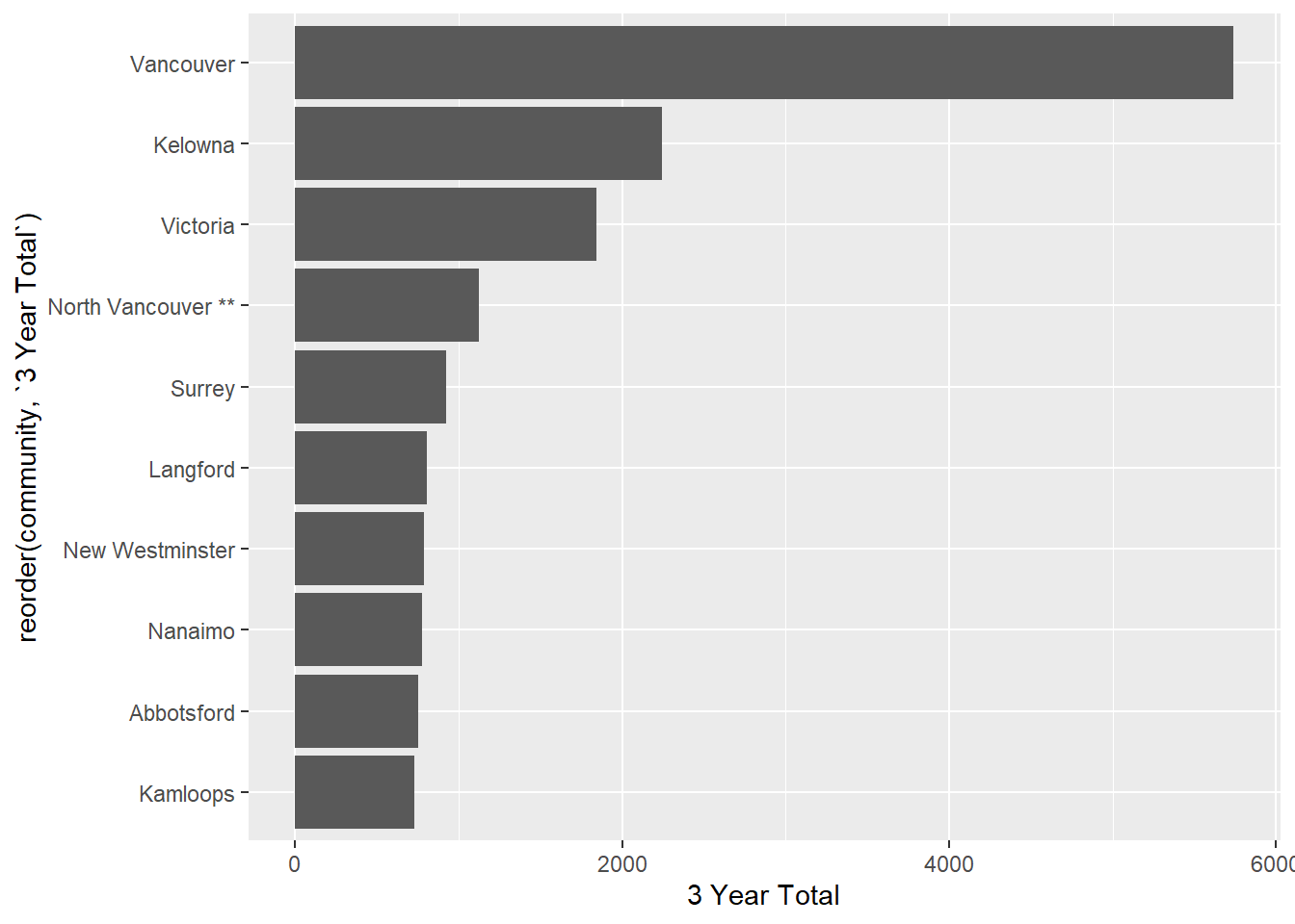
We can use our knowledge of regular expressions and the functions in {stringr} to remove these. The first thing we need to recall is that an asterisk is one of those Special characters{strings-special}, and we need to “escape” it with a backslash, and we need to escape the first backslash too. Here’s an example:
city_name <- "North Vancouver**"

# detect the presence of an asterisk
str_detect(city_name, "\\*")
## [1] TRUE
# detect the presence of an asterisk
str_count(city_name, "\\*")
## [1] 2{stringr} provides us functions for this very task:
str_remove()removes the first instance it finds, andstr_remove_all()removes all of them.
In a pipe with our dataframe, it would look like this:
housing1_long <- housing1_long |>
  mutate(community = str_remove_all(community, "\\*"))
Let’s filter for North Vancouver to check the success of our efforts:
housing1_long |>
  filter(community == "North Vancouver")
## # A tibble: 0 × 3
## # ℹ 3 variables: community <chr>, year <dbl>, units <dbl>What? Where are those rows? If we do a visual inspection, they are there. It turns out that there is a blank space between the community name and the asterisks.
There’s another {stringr} function for this: str_trim().
housing1_long <- housing1_long |>
  mutate(community = str_trim(community))

housing1_long |>
  filter(community == "North Vancouver")
## # A tibble: 3 × 3
## community year units
## <chr> <dbl> <dbl>
## 1 North Vancouver 2016 140
## 2 North Vancouver 2017 981
## 3 North Vancouver 2018 NAstr_trim()has an argumentside =if you need to specify left, right, or (the default) boththere is also a function
str_squish()that also takes out excess whitespace (it still does leading and trailing, likestr_trim())and if you need to add whitespace, there’s
str_pad()
Now our plot will have clean names:
ggplot(housing1_long |>
  group_by(community) |>
  tally(units, sort = TRUE, name = "3 Year Total") |>
  slice(1:10), aes(x = reorder(community, `3 Year Total`), y = `3 Year Total`))+
  geom_col() +
  coord_flip()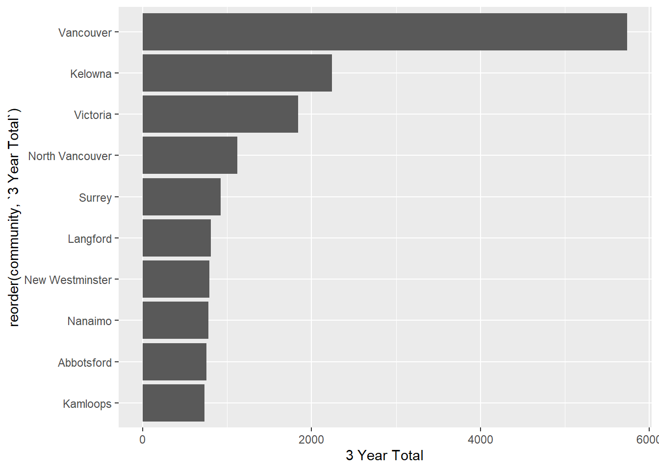
18.10.2 Splitting strings
This file has a single column, with both the name of every electoral district in British Columbia, preceded by a three-letter abbreviation (TLA).
bced <- read_csv("data/bc_electoral_districts_2015.txt", col_names = FALSE)
bced
## # A tibble: 87 × 1
## X1
## <chr>
## 1 "ABM\tAbbotsford-Mission"
## 2 "ABS\tAbbotsford South"
## 3 "ABW\tAbbotsford West"
## 4 "BDS\tBoundary-Similkameen"
## 5 "BND\tBurnaby-Deer Lake"
## 6 "BNE\tBurnaby-Edmonds"
## 7 "BNL\tBurnaby-Lougheed"
## 8 "BNN\tBurnaby North"
## 9 "CBC\tCariboo-Chilcotin"
## 10 "CBN\tCariboo North"
## # ℹ 77 more rowsYou’ll notice that in this file the three letter abbreviation is separated by “\t”. This is the regular expression for a tab.
From {stringr}, we can use the str_split() function:
## [[1]]
## [1] "ABM"                "Abbotsford-Mission"
##
## [[2]]
## [1] "ABS"              "Abbotsford South"
##
## [[3]]
## [1] "ABW"             "Abbotsford West"
##
## [[4]]
## [1] "BDS"                  "Boundary-Similkameen"
##
## [[5]]
## [1] "BND"               "Burnaby-Deer Lake"
##
## [[6]]
## [1] "BNE"             "Burnaby-Edmonds"
But there’s a solution designed for tabular data, in the {tidyr} package: separate()
## # A tibble: 87 × 2
##    ed_tla ed_name
##    <chr>  <chr>
##  1 ABM    Abbotsford-Mission
##  2 ABS    Abbotsford South
##  3 ABW    Abbotsford West
##  4 BDS    Boundary-Similkameen
##  5 BND    Burnaby-Deer Lake
##  6 BNE    Burnaby-Edmonds
##  7 BNL    Burnaby-Lougheed
##  8 BNN    Burnaby North
##  9 CBC    Cariboo-Chilcotin
## 10 CBN    Cariboo North
## # ℹ 77 more rows
If we add the remove = argument set to FALSE, the original variable remains:
## # A tibble: 87 × 3
##    X1                          ed_tla ed_name
##    <chr>                       <chr>  <chr>
##  1 "ABM\tAbbotsford-Mission"   ABM    Abbotsford-Mission
##  2 "ABS\tAbbotsford South"     ABS    Abbotsford South
##  3 "ABW\tAbbotsford West"      ABW    Abbotsford West
##  4 "BDS\tBoundary-Similkameen" BDS    Boundary-Similkameen
##  5 "BND\tBurnaby-Deer Lake"    BND    Burnaby-Deer Lake
##  6 "BNE\tBurnaby-Edmonds"      BNE    Burnaby-Edmonds
##  7 "BNL\tBurnaby-Lougheed"     BNL    Burnaby-Lougheed
##  8 "BNN\tBurnaby North"        BNN    Burnaby North
##  9 "CBC\tCariboo-Chilcotin"    CBC    Cariboo-Chilcotin
## 10 "CBN\tCariboo North"        CBN    Cariboo North
## # ℹ 77 more rows
In the above example, the tab symbol is the separator, and there’s only one per line. But what if the abbreviation and the name were separated by spaces? In that case, we would want to separate on only the first space.
bced_space <- read_csv("data/bc_electoral_districts_2015_space.txt", col_names = FALSE)
bced_space
## # A tibble: 87 × 1
## X1
## <chr>
## 1 ABM Abbotsford-Mission
## 2 ABS Abbotsford South
## 3 ABW Abbotsford West
## 4 BDS Boundary-Similkameen
## 5 BND Burnaby-Deer Lake
## 6 BNE Burnaby-Edmonds
## 7 BNL Burnaby-Lougheed
## 8 BNN Burnaby North
## 9 CBC Cariboo-Chilcotin
## 10 CBN Cariboo North
## # ℹ 77 more rows## # A tibble: 87 × 2
## ed_tla ed_name
## <chr> <chr>
## 1 ABM Abbotsford-Mission
## 2 ABS Abbotsford
## 3 ABW Abbotsford
## 4 BDS Boundary-Similkameen
## 5 BND Burnaby-Deer
## 6 BNE Burnaby-Edmonds
## 7 BNL Burnaby-Lougheed
## 8 BNN Burnaby
## 9 CBC Cariboo-Chilcotin
## 10 CBN Cariboo
## # ℹ 77 more rowsFor the electoral districts with only a single word or a hyphen, it works fine. But notice that the two Abbotsford ridings are now just “Abbotsford”, since everything after the second space has been dropped.
The solution is to use the extra = "merge" argument. (Note that the default is extra = "drop".)
## # A tibble: 87 × 2
##    ed_tla ed_name
##    <chr>  <chr>
##  1 ABM    Abbotsford-Mission
##  2 ABS    Abbotsford South
##  3 ABW    Abbotsford West
##  4 BDS    Boundary-Similkameen
##  5 BND    Burnaby-Deer Lake
##  6 BNE    Burnaby-Edmonds
##  7 BNL    Burnaby-Lougheed
##  8 BNN    Burnaby North
##  9 CBC    Cariboo-Chilcotin
## 10 CBN    Cariboo North
## # ℹ 77 more rows
Nice!
-30-