9 R Markdown
9.1 Setup
This chunk of R code loads the packages that we will be using.
This document will introduce you to R Markdown notebooks, and give you some hands-on experience adding to the document.
9.2 Reading & reference
Garrett Grolemund and Hadley Wickham, R for Data Science, 1st ed.
Yihui Xie, Christophe Dervieux, Emily Riederer, R Markdown Cookbook
R Markdown: Get Started—a series of short lessons on R Markdown
The R Markdown cheatsheet and reference guide, available online and through the “Help / Cheatsheets >” menu item in RStudio
Yihui Xie, J. J. Allaire, Garrett Grolemund, R Markdown: The Definitive Guide(Yihui Xie and Grolemund 2019)
- code chunk options described here: https://bookdown.org/yihui/rmarkdown/r-code.html
9.3 Getting started
You can create a new R Markdown document in RStudio by clicking the menu item:
- File / New File > R Notebook
or
- File / New File > R Markdown…
For this course, we will be using the Document option…for your project, you may wish to use another format.
9.3.1 Typing, running, and knitting
When you type in an R Markdown document, you just get what you type.
The magic starts to happen when you run R code chunks in the document…we will get to that soon.
And the real whiz-bang thing is that when you’ve finished, you can “knit” the document. At that point, the code chunks are run, and the markdown formatting is interpreted, and you get a beautiful document.
9.4 Markdown syntax
Markdown is a great way to write a report, slide deck, book, … even hands-on exercises for a class!
Formatting is simple. Check the cheatsheet for some details, or this section of R for Data Science
9.4.0.1 Your Turn
Write something that you want bolded:
Now, make a bullet list with the names of three colours:
Add a hypertext link to the text book’s title: Hadley Wickham and Garrett Grolemund, R for Data Science, so that it creates a link to the online version of the book at r4ds.had.co.nz .
Add an image of the data science process…the file is “data-science.png”

9.5 The first chunk: “setup”
It’s good practice to load all of the packages you’ll require at the top of your script. When a package is loaded, all of the functions and data in the package are available.
Loading an installed package is done with the library() function. The R chunk named “setup” will load the {tidyverse} package (which in turn will load other packages, such as the data manipulation package {dplyr} and the plotting package {ggplot2}).
To run a chunk, press the green arrow at the far right of the chunk, or put your cursor in the chunk and press Ctrl + Shift + Enter (on macOS, Cmd + Shift + Enter)
9.5.1 Your Turn
Add the package {cowsay} to the setup chunk, and run the chunk.
- Add a new chunk to the R Markdown document.
You can do this with the “Insert” toolbar button, or the keyboard shortcut
Ctrl + Alt + ICmd + Option + Ion macOS
You could also type the three back ticks, the curly braces, the letter R, and three more backticks to end the chunk–but that’s a very WET approach!
- Name the chunk so that you can navigate to it later.
In the new chunk you have just created, type the function say() (which is from the {cowsay} package), inside the parentheses put a short quote (for example, “I like DAMS302”), and then run the chunk…
# solution

say("I like DAMS302")
9.5.2 Getting help
Now, type ?say in the console to activate the Help menu for this function. Try some of the other arguments. (Note that an important by = option is not listed: “yoda”.)
Try experimenting with other arguments. For example, instead of your quote (which is the what = argument), you could put what = "time".
Now you have had a chance to experiment with that silliness…onward!
9.6 Chunk contents
Code chunks can create an object, which is stored in the Global Environment…it will be listed under the “Environment” tab in the top right of your RStudio screen.
That object can then be referenced in a future chunk and in inline text. This can be very useful!
9.6.1 Your Turn
Use the seq() function to create an object “my_numbers” that contains the integers from 3 to 7.
If you’re not sure about the syntax of the function, don’t hesitate to use the ?seq command in the console…
# solution
my_numbers <- seq(from = 3, to = 7)
Now, use the next chunk to calculate the sum of the numbers in my_numbers. Assign the sum to an object my_total, and print the total.
# solution
my_total <- sum(my_numbers)
my_total
## [1] 25R code chunks can contain anything you want to do in R.
Here’s a chunk that contains code to create a chart from everyone’s favourite data set, penguins (from the {palmerpenguins} package).
Run the chunk and see what happens…
ggplot(data = penguins) +
  geom_point(mapping = aes(x = body_mass_g, y = flipper_length_mm))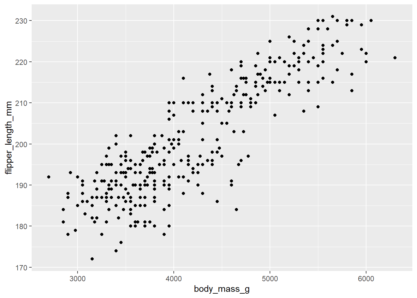
9.7 Inline R code
R Markdown allows you to insert a calculated value into the middle of your text. This is accomplished by putting a single backtick followed by the letter “r” (lower case, with no space after the backtick) and then your code, and ended with another backtick.
Here’s an example: to calculate the radius of a circle, we could write an R code chunk with the following code:
pi * 3^2## [1] 28.27433Or we could put that calculation inside a sentence. When this document is “knit”, the code will be evaluated, and the result inserted into the text.
The area of a circle with a radius of 3 mm is 28.2743339 sq. mm.
Now is your chance to get fancy: write a sentence that uses inline code and the function sqrt to calculate the square root of my_total, which you calculated before.
9.8 Rendering the HTML file
At this point, we want to knit it all together.
9.8.1 Your Turn - rendering the HTML file
Below is that chunk from above that creates a chart. When we are rendering the final document, we might not want to have the code displayed (it might be a fancy report for your boss’s boss)—we just want the chart.
The solution is to use one of many code chunk options that are available. These options control how the chunk is interpreted…you can leave the code visible but not run at all, or to omit rendering any messages that might clutter your output.
ggplot(data = mpg) +
  geom_point(mapping = aes(x = displ, y = hwy))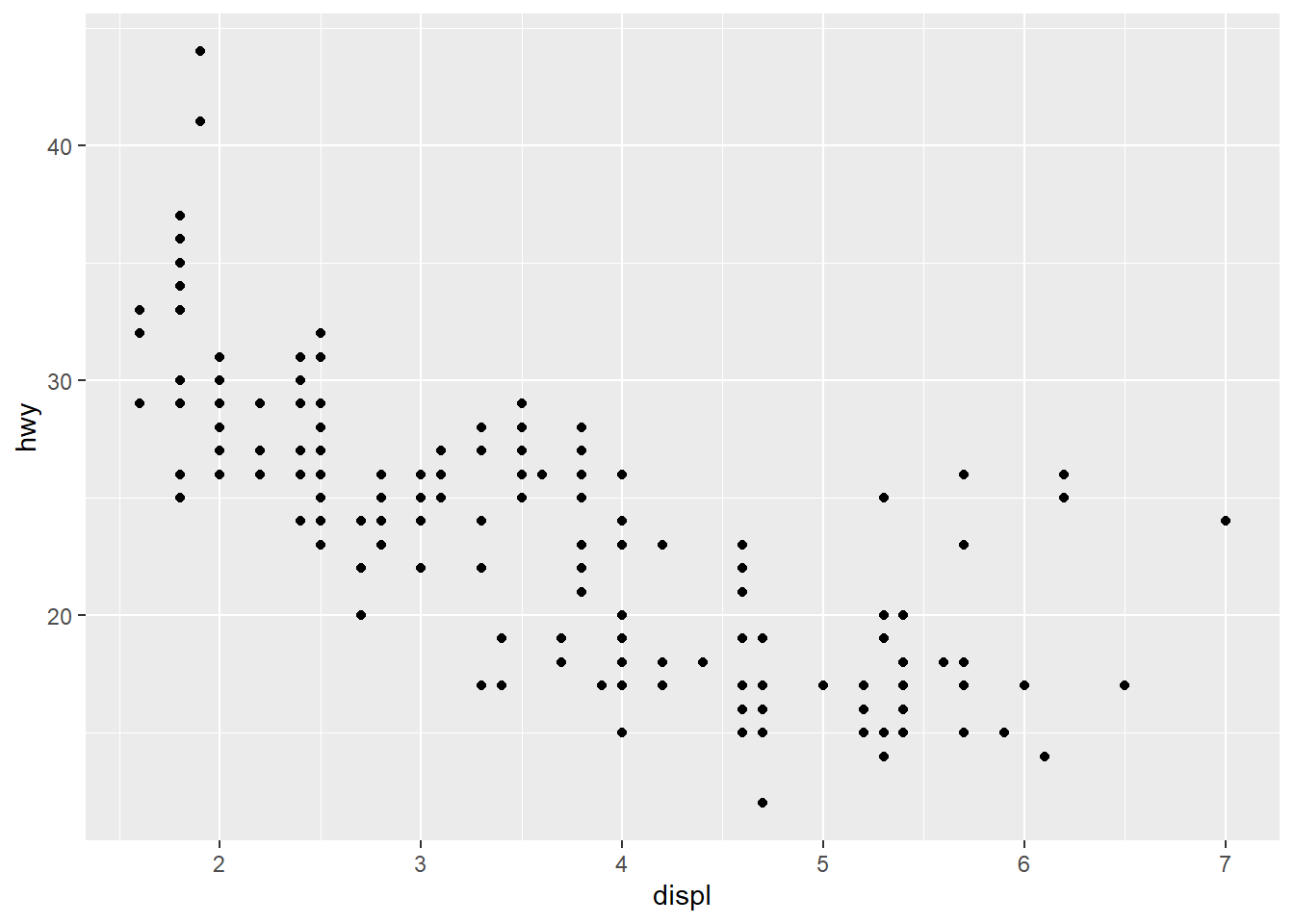
The solution is to put the option “echo = FALSE” after the “r” in the opening bit of the code. There are other options for the chunks that you may find useful.
9.9 The YAML
When we started our new R markdown file, there is a chunk of text at the top that we’ve ignored so far. This is the YAML (which now stands for “YAML Ain’t Markup Language”.)
The YAML contents gives us the opportunity to control what happens when we knit our document.
For example, there are a variety of themes, which you can find listed at the Bootstrap site.
What happens when you replace the output: html_document with the following?
output:
  html_document:
    theme: united
    highlight: tango
9.9.1 Table of contents
You can add a table of contents with
output:
  html_document:
    toc: true
One of my favourites is the floating table of contents:
output:
  html_document:
    toc: true
    toc_float: true
More about the table of contents here: https://bookdown.org/yihui/rmarkdown/html-document.html#table-of-contents
9.9.2 Output formats
You can change the type of document being output. The current setting for this file is output: html_document. But by changing it to output: word_document, the result of knitting is a Word format document!
The full list of output formats can be found here: https://bookdown.org/yihui/rmarkdown/output-formats.html
-30-