14 Relational data
14.1 Objectives
understand the function of keys in relational databases
understand how to join tables
understand the primary types of mutating and filtering joins
14.3 Reading
This hands-on exercise draws heavily on the following sources:
Another resource with a good explanation of the types of joins can be found at [Tidy Animated Verbs}(https://www.garrickadenbuie.com/project/tidyexplain/)(Aden‑Buie 2021)
For some additional examples of table joins, see William Surles, Joining Data in R with dplyr
14.4 Relational data
Often, the data you are working with are spread across multiple tables. This allows for efficient database storage (there’s an entire discipline dedicated to database theory and practical implementations of those theories.)
This requires you, the data analyst, to join tables, so that the information held in multiple tables can be used to answer the research question at hand.
Earlier you worked with the {nycflights13} package; for this hands-on exercise we will return to it.
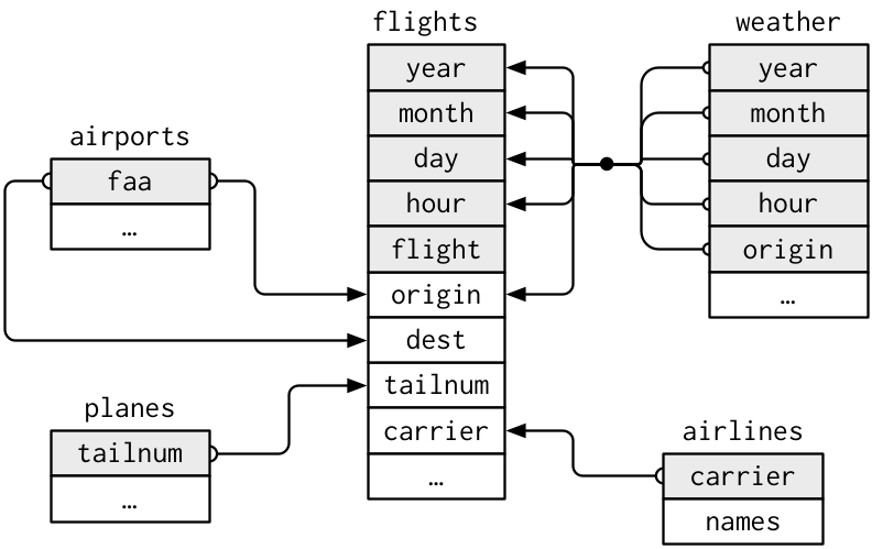
In addition to flights, there are four other tables in the package:
airlinesairportsplanesweather
The tables are related to flights by the fact that they have variables in common. These are known as the “key” variables.
This diagram shows the relationships:
14.5 Keys
Primary: identifies a unique observation in the table.
Foreign: a unique observation in another table, but not this one.
An example: tailnum
primary in
planes– there is only one observation for each aircraftforeign in
flights– a plane could have multiple flights in and out of NYC airports
Having the same key in two tables forms the “relation” – hence “relational database”.
14.5.0.1 Your turn
Use count to check that planes$tailnum is a primary key
Solution
## # A tibble: 0 × 2
## # ℹ 2 variables: tailnum <chr>, n <int>## # A tibble: 1 × 1
## `max(n)`
## <int>
## 1 1## # A tibble: 4,044 × 2
## tailnum n
## <chr> <int>
## 1 D942DN 4
## 2 N0EGMQ 371
## 3 N10156 153
## 4 N102UW 48
## 5 N103US 46
## 6 N104UW 47
## 7 N10575 289
## 8 N105UW 45
## 9 N107US 41
## 10 N108UW 60
## # ℹ 4,034 more rowsSometimes tables don’t have a primary key! When that happens, it can be useful to create one: mutate() and row_number() is one approach. This is a surrogate key.
14.6 Mutating joins
The first kind of joins are “mutating joins”—new variables are added to one data frame from matching observations in another.
14.6.1 Understanding keys
-
adapted from from _R for Data Science, “Understanding joins”
- In particular, you may wish to review the visual representations at “Understanding joins”
First, we will make two small tables, table_one and table_two
14.6.2 Inner joins
An inner join keeps only the observations where there is a match on both sides. The key variables is identified using the by = argument:
inner_join(x = table_one, y = table_two, by = "key_var")## # A tibble: 2 × 3
## key_var colour_t1 fruit_t2
## <chr> <chr> <chr>
## 1 key1 red apple
## 2 key2 blue blueberryNote that in the circumstances where we are confident that the key variables are named the same in both tables, we can use a bit of coding short-hand and omit the by = argument. You will see a message in the console (and your R markdown thumbnail) letting you know what variables are used for the join.
inner_join(table_one, table_two)## # A tibble: 2 × 3
## key_var colour_t1 fruit_t2
## <chr> <chr> <chr>
## 1 key1 red apple
## 2 key2 blue blueberry14.6.3 Left join
Left, right, and full joins are varieties of “outer joins”.
Join the two tables using a left join: … all of the observations from the first table (on the left-hand side of the function), and variables from the matching records from the secon (the right-hand side of the function).
The {dplyr} function for this is left_join()
left_join(table_one, table_two, by = "key_var")## # A tibble: 3 × 3
## key_var colour_t1 fruit_t2
## <chr> <chr> <chr>
## 1 key1 red apple
## 2 key2 blue blueberry
## 3 key3 yellow <NA>Note that all 3 of the table_one values are there; because there is no table_two observation with the key value of “key3”, the fruit_t2 value is NA.
right join
Is the same as a left join, but keeps all of the observations in the right-hand table y
full join
Keeps all of the observations in both x and y
See what happens when you join the tables with a right_join(), followed by a full_join()
# solution
right_join(table_one, table_two, by = "key_var")## # A tibble: 3 × 3
## key_var colour_t1 fruit_t2
## <chr> <chr> <chr>
## 1 key1 red apple
## 2 key2 blue blueberry
## 3 key4 <NA> banana
full_join(table_one, table_two, by = "key_var")## # A tibble: 4 × 3
## key_var colour_t1 fruit_t2
## <chr> <chr> <chr>
## 1 key1 red apple
## 2 key2 blue blueberry
## 3 key3 yellow <NA>
## 4 key4 <NA> banana14.6.3.1 Your turn
In this example, we will add the name of the airline to the flights table. First, we will make a smaller version of the flights table by selecting a few of the variables, and taking the first 100 rows with the slice() function (see https://dplyr.tidyverse.org/reference/slice.html).
flights2 <- flights |>
select(year:day, hour, origin, dest, tailnum, carrier) |>
slice(1:100)
flights2## # A tibble: 100 × 8
## year month day hour origin dest tailnum carrier
## <int> <int> <int> <dbl> <chr> <chr> <chr> <chr>
## 1 2013 1 1 5 EWR IAH N14228 UA
## 2 2013 1 1 5 LGA IAH N24211 UA
## 3 2013 1 1 5 JFK MIA N619AA AA
## 4 2013 1 1 5 JFK BQN N804JB B6
## 5 2013 1 1 6 LGA ATL N668DN DL
## 6 2013 1 1 5 EWR ORD N39463 UA
## 7 2013 1 1 6 EWR FLL N516JB B6
## 8 2013 1 1 6 LGA IAD N829AS EV
## 9 2013 1 1 6 JFK MCO N593JB B6
## 10 2013 1 1 6 LGA ORD N3ALAA AA
## # ℹ 90 more rowsTo this table we will add the name of the airline, which we can find in the table airlines.
both tables have the variable “carrier”
we want a
left_join: all theflightobservations, and adding the “name” variable fromairlines
Solution
# solution
left_join(flights2, airlines, by = "carrier")## # A tibble: 100 × 9
## year month day hour origin dest tailnum carrier name
## <int> <int> <int> <dbl> <chr> <chr> <chr> <chr> <chr>
## 1 2013 1 1 5 EWR IAH N14228 UA United Air Lines Inc.
## 2 2013 1 1 5 LGA IAH N24211 UA United Air Lines Inc.
## 3 2013 1 1 5 JFK MIA N619AA AA American Airlines Inc.
## 4 2013 1 1 5 JFK BQN N804JB B6 JetBlue Airways
## 5 2013 1 1 6 LGA ATL N668DN DL Delta Air Lines Inc.
## 6 2013 1 1 5 EWR ORD N39463 UA United Air Lines Inc.
## 7 2013 1 1 6 EWR FLL N516JB B6 JetBlue Airways
## 8 2013 1 1 6 LGA IAD N829AS EV ExpressJet Airlines Inc.
## 9 2013 1 1 6 JFK MCO N593JB B6 JetBlue Airways
## 10 2013 1 1 6 LGA ORD N3ALAA AA American Airlines Inc.
## # ℹ 90 more rowsUsing a pipe, the same result can be achieved with the following:
# alternate version, using a pipe
flights2 |>
left_join(airlines, by = "carrier")## # A tibble: 100 × 9
## year month day hour origin dest tailnum carrier name
## <int> <int> <int> <dbl> <chr> <chr> <chr> <chr> <chr>
## 1 2013 1 1 5 EWR IAH N14228 UA United Air Lines Inc.
## 2 2013 1 1 5 LGA IAH N24211 UA United Air Lines Inc.
## 3 2013 1 1 5 JFK MIA N619AA AA American Airlines Inc.
## 4 2013 1 1 5 JFK BQN N804JB B6 JetBlue Airways
## 5 2013 1 1 6 LGA ATL N668DN DL Delta Air Lines Inc.
## 6 2013 1 1 5 EWR ORD N39463 UA United Air Lines Inc.
## 7 2013 1 1 6 EWR FLL N516JB B6 JetBlue Airways
## 8 2013 1 1 6 LGA IAD N829AS EV ExpressJet Airlines Inc.
## 9 2013 1 1 6 JFK MCO N593JB B6 JetBlue Airways
## 10 2013 1 1 6 LGA ORD N3ALAA AA American Airlines Inc.
## # ℹ 90 more rowsHere’s an example of where the utility of the pipe operator can be seen. If we want to count the number of flights be each airline, we could use the “carrier” variable, which is the short code. But a more useful table would have the airline name. In this code, the join is followed by a group_by and then tally(), which produces a table with the airline name.
## # A tibble: 11 × 2
## name n
## <chr> <int>
## 1 AirTran Airways Corporation 1
## 2 Alaska Airlines Inc. 1
## 3 American Airlines Inc. 17
## 4 Delta Air Lines Inc. 13
## 5 Envoy Air 6
## 6 ExpressJet Airlines Inc. 3
## 7 JetBlue Airways 25
## 8 Southwest Airlines Co. 1
## 9 US Airways Inc. 5
## 10 United Air Lines Inc. 26
## 11 Virgin America 214.6.4 Duplicate Keys
In real life, tables start to get more complex. It’s often the case that you will have tables that have duplicate keys in one or both of the tables.
The chunk below creates new tables table_a and table_b, where there are duplicate keys in one.
table_a <- tribble(~ key_var, ~ day_a,
"key1", "Mon",
"key1", "Tue",
"key2", "Wed",
"key2", "Thu")
table_b <- tribble(~ key_var, ~ veg_b,
"key1", "carrot",
"key2", "tomato")14.6.4.1 Your turn
Join the tables with left_join(), with a as the table on the left.
Solution
# solution
left_join(table_a, table_b, by = "key_var")## # A tibble: 4 × 3
## key_var day_a veg_b
## <chr> <chr> <chr>
## 1 key1 Mon carrot
## 2 key1 Tue carrot
## 3 key2 Wed tomato
## 4 key2 Thu tomatoIn this example, where the duplicates are on the left, the same value “carrot” gets joined to both “key1” cases.
A situation where there are duplicate keys in both tables is usually an error—there is no unique identifier of a single observation. (A question to ask yourself is “Is there are third table?”)
14.6.4.2 Your turn
Here’s different tables, where the key “key2” is duplicated in both.
table_m <- tribble(~ key_var, ~ month_m,
"key1", "Jan",
"key2", "Feb",
"key2", "Mar")
table_n <- tribble(~ key_var, ~ ball_n,
"key1", "foot",
"key2", "basket",
"key2", "base")What does a left join do? How many rows does the resulting table have?
Solution
# solution
left_join(table_m, table_n, by = "key_var")## # A tibble: 5 × 3
## key_var month_m ball_n
## <chr> <chr> <chr>
## 1 key1 Jan foot
## 2 key2 Feb basket
## 3 key2 Feb base
## 4 key2 Mar basket
## 5 key2 Mar baseThe left_join() function adds both “basket” and “base” to each of the “Feb” and “Mar” records on the left. This leads to a duplication of the rows with “key2”—so the whole table jumps from 3 rows (what we would expect with a left_join()) to 5 rows.
14.7 Filtering joins
The other sort of joins filter observations from one data frame based on whether or not they match an observation in the other table.
There are two sorts:
semi_join(x, y)keeps all observations inxthat have a match iny.anti_join(x, y)drops all observations inxthat have a match iny.
Let’s go back to our original test tables again:
table_one <- tribble(
~key_var, ~colour_t1,
"key1", "red",
"key2", "blue",
"key3", "yellow"
)
table_two <- tribble(
~key_var, ~fruit_t2,
"key1", "apple",
"key2", "blueberry",
"key4", "banana"
)Semi-join: only the observations in x that have a match in y.
Note that no variables from y appear in the result.
semi_join(table_one, table_two, by = "key_var")## # A tibble: 2 × 2
## key_var colour_t1
## <chr> <chr>
## 1 key1 red
## 2 key2 blueAnti-join: returns the observations in x that don’t have a key match in y. Again, no values from y appear in the result.
anti_join(table_one, table_two, by = "key_var")## # A tibble: 1 × 2
## key_var colour_t1
## <chr> <chr>
## 1 key3 yellow14.8 More complex scenarios
14.8.1 Keys with different names
In some circumstances, you will encounter a situation where your key variables are named one thing in one table, and something quite different in another.
Here is a solution. In this example, the key variable in one table is named key_x and in the other it is key_y.
left_tbl <- tribble(
~key_x, ~val_x,
1, "x1",
2, "x2",
3, "x3"
)
right_tbl <- tribble(
~key_y, ~val_y, ~val_y2,
1, "y1", "Monday",
2, "y2", "Tuesday",
4, "y3", "Wednesday"
)Here are two different ways of writing the same code:
# to specify key variables with different names:
left_join(left_tbl, right_tbl, by = c("key_x" = "key_y"))## # A tibble: 3 × 4
## key_x val_x val_y val_y2
## <dbl> <chr> <chr> <chr>
## 1 1 x1 y1 Monday
## 2 2 x2 y2 Tuesday
## 3 3 x3 <NA> <NA>## # A tibble: 3 × 4
## key_x val_x val_y val_y2
## <dbl> <chr> <chr> <chr>
## 1 1 x1 y1 Monday
## 2 2 x2 y2 Tuesday
## 3 3 x3 <NA> <NA>14.8.2 Join on multiple keys
In the {nycflights13} database (that is, the multiple related tables), we see that the “flights” table is linked to the “weather” table on five different variables. The “weather” table holds the primary key, where there is a unique row by the five variables “year”, “month”, “day”, “hour”, and “origin” (with the airport code).
head(weather)## # A tibble: 6 × 15
## origin year month day hour temp dewp humid wind_dir wind_speed wind_gust precip pressure
## <chr> <int> <int> <int> <int> <dbl> <dbl> <dbl> <dbl> <dbl> <dbl> <dbl> <dbl>
## 1 EWR 2013 1 1 1 39.0 26.1 59.4 270 10.4 NA 0 1012
## 2 EWR 2013 1 1 2 39.0 27.0 61.6 250 8.06 NA 0 1012.
## 3 EWR 2013 1 1 3 39.0 28.0 64.4 240 11.5 NA 0 1012.
## 4 EWR 2013 1 1 4 39.9 28.0 62.2 250 12.7 NA 0 1012.
## 5 EWR 2013 1 1 5 39.0 28.0 64.4 260 12.7 NA 0 1012.
## 6 EWR 2013 1 1 6 37.9 28.0 67.2 240 11.5 NA 0 1012.
## # ℹ 2 more variables: visib <dbl>, time_hour <dttm>If we were analyzing the relationship between flight departure delays (in the “flights” table) and weather conditions, we would need to link these tables.
The first solution is to name all of the variables inside a by = c() argument.
## # A tibble: 336,776 × 29
## year month day dep_time sched_dep_time dep_delay arr_time sched_arr_time arr_delay carrier
## <int> <int> <int> <int> <int> <dbl> <int> <int> <dbl> <chr>
## 1 2013 1 1 517 515 2 830 819 11 UA
## 2 2013 1 1 533 529 4 850 830 20 UA
## 3 2013 1 1 542 540 2 923 850 33 AA
## 4 2013 1 1 544 545 -1 1004 1022 -18 B6
## 5 2013 1 1 554 600 -6 812 837 -25 DL
## 6 2013 1 1 554 558 -4 740 728 12 UA
## 7 2013 1 1 555 600 -5 913 854 19 B6
## 8 2013 1 1 557 600 -3 709 723 -14 EV
## 9 2013 1 1 557 600 -3 838 846 -8 B6
## 10 2013 1 1 558 600 -2 753 745 8 AA
## # ℹ 336,766 more rows
## # ℹ 19 more variables: flight <int>, tailnum <chr>, origin <chr>, dest <chr>, air_time <dbl>,
## # distance <dbl>, hour <dbl>, minute <dbl>, time_hour.x <dttm>, temp <dbl>, dewp <dbl>,
## # humid <dbl>, wind_dir <dbl>, wind_speed <dbl>, wind_gust <dbl>, precip <dbl>, pressure <dbl>,
## # visib <dbl>, time_hour.y <dttm>In this second approach, the range of variables is specified with the : operator. Note that this is now inside a pipe, and the left table (“flights”) is named at the top of the pipe sequence.
left_join(flights, weather)## # A tibble: 336,776 × 28
## year month day dep_time sched_dep_time dep_delay arr_time sched_arr_time arr_delay carrier
## <int> <int> <int> <int> <int> <dbl> <int> <int> <dbl> <chr>
## 1 2013 1 1 517 515 2 830 819 11 UA
## 2 2013 1 1 533 529 4 850 830 20 UA
## 3 2013 1 1 542 540 2 923 850 33 AA
## 4 2013 1 1 544 545 -1 1004 1022 -18 B6
## 5 2013 1 1 554 600 -6 812 837 -25 DL
## 6 2013 1 1 554 558 -4 740 728 12 UA
## 7 2013 1 1 555 600 -5 913 854 19 B6
## 8 2013 1 1 557 600 -3 709 723 -14 EV
## 9 2013 1 1 557 600 -3 838 846 -8 B6
## 10 2013 1 1 558 600 -2 753 745 8 AA
## # ℹ 336,766 more rows
## # ℹ 18 more variables: flight <int>, tailnum <chr>, origin <chr>, dest <chr>, air_time <dbl>,
## # distance <dbl>, hour <dbl>, minute <dbl>, time_hour <dttm>, temp <dbl>, dewp <dbl>,
## # humid <dbl>, wind_dir <dbl>, wind_speed <dbl>, wind_gust <dbl>, precip <dbl>, pressure <dbl>,
## # visib <dbl>## # A tibble: 336,776 × 20
## year month day dep_time sched_dep_time dep_delay arr_time sched_arr_time arr_delay carrier
## <int> <int> <int> <int> <int> <dbl> <int> <int> <dbl> <chr>
## 1 2013 1 1 517 515 2 830 819 11 UA
## 2 2013 1 1 533 529 4 850 830 20 UA
## 3 2013 1 1 542 540 2 923 850 33 AA
## 4 2013 1 1 544 545 -1 1004 1022 -18 B6
## 5 2013 1 1 554 600 -6 812 837 -25 DL
## 6 2013 1 1 554 558 -4 740 728 12 UA
## 7 2013 1 1 555 600 -5 913 854 19 B6
## 8 2013 1 1 557 600 -3 709 723 -14 EV
## 9 2013 1 1 557 600 -3 838 846 -8 B6
## 10 2013 1 1 558 600 -2 753 745 8 AA
## # ℹ 336,766 more rows
## # ℹ 10 more variables: flight <int>, tailnum <chr>, origin <chr>, dest <chr>, air_time <dbl>,
## # distance <dbl>, hour <dbl>, minute <dbl>, time_hour <dttm>, temp <dbl>14.8.3 Select specific columns
Using our left_tbl and right_tbl from above, here is a solution that embeds a pipe and select function inside the right_tbl call. Note that the comma follows the select(), not the name of the table.
# to specify variables to add to new table
# one solution: put select in the table naming
full_join(left_tbl,
right_tbl |> select(key_y, val_y2),
by = c("key_x" = "key_y"))## # A tibble: 4 × 3
## key_x val_x val_y2
## <dbl> <chr> <chr>
## 1 1 x1 Monday
## 2 2 x2 Tuesday
## 3 3 x3 <NA>
## 4 4 <NA> WednesdayIn the {nycflights13} case, where we are joining on multiple keys and then wanting just the temperature variable from the right (“weather”) table, here are three different left_join() solutions:
# solution
flights |>
left_join(weather |> select("year", "month", "day", "hour", "origin", "temp"),
by = c("year", "month", "day", "hour", "origin"))## # A tibble: 336,776 × 20
## year month day dep_time sched_dep_time dep_delay arr_time sched_arr_time arr_delay carrier
## <int> <int> <int> <int> <int> <dbl> <int> <int> <dbl> <chr>
## 1 2013 1 1 517 515 2 830 819 11 UA
## 2 2013 1 1 533 529 4 850 830 20 UA
## 3 2013 1 1 542 540 2 923 850 33 AA
## 4 2013 1 1 544 545 -1 1004 1022 -18 B6
## 5 2013 1 1 554 600 -6 812 837 -25 DL
## 6 2013 1 1 554 558 -4 740 728 12 UA
## 7 2013 1 1 555 600 -5 913 854 19 B6
## 8 2013 1 1 557 600 -3 709 723 -14 EV
## 9 2013 1 1 557 600 -3 838 846 -8 B6
## 10 2013 1 1 558 600 -2 753 745 8 AA
## # ℹ 336,766 more rows
## # ℹ 10 more variables: flight <int>, tailnum <chr>, origin <chr>, dest <chr>, air_time <dbl>,
## # distance <dbl>, hour <dbl>, minute <dbl>, time_hour <dttm>, temp <dbl>
# slightly different syntax:
flights |>
left_join(select(weather, "year", "month", "day", "hour", "origin", "temp"),
by = c("year", "month", "day", "hour", "origin"))## # A tibble: 336,776 × 20
## year month day dep_time sched_dep_time dep_delay arr_time sched_arr_time arr_delay carrier
## <int> <int> <int> <int> <int> <dbl> <int> <int> <dbl> <chr>
## 1 2013 1 1 517 515 2 830 819 11 UA
## 2 2013 1 1 533 529 4 850 830 20 UA
## 3 2013 1 1 542 540 2 923 850 33 AA
## 4 2013 1 1 544 545 -1 1004 1022 -18 B6
## 5 2013 1 1 554 600 -6 812 837 -25 DL
## 6 2013 1 1 554 558 -4 740 728 12 UA
## 7 2013 1 1 555 600 -5 913 854 19 B6
## 8 2013 1 1 557 600 -3 709 723 -14 EV
## 9 2013 1 1 557 600 -3 838 846 -8 B6
## 10 2013 1 1 558 600 -2 753 745 8 AA
## # ℹ 336,766 more rows
## # ℹ 10 more variables: flight <int>, tailnum <chr>, origin <chr>, dest <chr>, air_time <dbl>,
## # distance <dbl>, hour <dbl>, minute <dbl>, time_hour <dttm>, temp <dbl>
# let {dplyr} decide the variables on which to join
flights |>
left_join(select(weather, origin:temp))## # A tibble: 336,776 × 20
## year month day dep_time sched_dep_time dep_delay arr_time sched_arr_time arr_delay carrier
## <int> <int> <int> <int> <int> <dbl> <int> <int> <dbl> <chr>
## 1 2013 1 1 517 515 2 830 819 11 UA
## 2 2013 1 1 533 529 4 850 830 20 UA
## 3 2013 1 1 542 540 2 923 850 33 AA
## 4 2013 1 1 544 545 -1 1004 1022 -18 B6
## 5 2013 1 1 554 600 -6 812 837 -25 DL
## 6 2013 1 1 554 558 -4 740 728 12 UA
## 7 2013 1 1 555 600 -5 913 854 19 B6
## 8 2013 1 1 557 600 -3 709 723 -14 EV
## 9 2013 1 1 557 600 -3 838 846 -8 B6
## 10 2013 1 1 558 600 -2 753 745 8 AA
## # ℹ 336,766 more rows
## # ℹ 10 more variables: flight <int>, tailnum <chr>, origin <chr>, dest <chr>, air_time <dbl>,
## # distance <dbl>, hour <dbl>, minute <dbl>, time_hour <dttm>, temp <dbl>14.8.4 Non-key variables with the same names
Here’s another case—let’s imagine we have two tables, called “orders” and “shipments”. They have two variables with the same names, “order_number” and “dollar_value”. The “order_number” is a unique ID (the key variable), but the dollars associated with the order might be different than the shipment—sometimes items are out of stock, so they can’t be sent, so the value of the shipment is less than what was ordered.
orders <- tribble(
~order_number, ~dollar_value,
"x1", 11,
"x2", 12,
"x3", 13,
"x4", 14
)
shipments <- tribble(
~order_number, ~dollar_value,
"x1", 11,
"x2", 11,
"x3", 13,
"x4", 4
)When we join the tables, we will use “order_number” to join them. There will be only one column in the resulting dataframe with this name.
A variable called “dollar_value” exists in both tables, but means different things. You and I know that one could be called “dollar_value_orders” and the other “dollar_value_shipments”—but R doesn’t know that, so it renames them “dollar_value.x” and “dollar_value.y”. The one with the “.x” at the end will be the left table, and “.y” will be the right table.
orders_shipped <- orders |>
full_join(shipments, by = "order_number")
orders_shipped## # A tibble: 4 × 3
## order_number dollar_value.x dollar_value.y
## <chr> <dbl> <dbl>
## 1 x1 11 11
## 2 x2 12 11
## 3 x3 13 13
## 4 x4 14 4You could then rename “dollar_value.x” and “dollar_value.y” to make it clear which is which. In this example, we also then add a column showing the percentage of the original order that was shipped.
orders_shipped |>
rename("dollar_value_order" = dollar_value.x,
"dollar_value_shipment" = dollar_value.y) |>
mutate(filled_pct = round((dollar_value_shipment / dollar_value_order) *100, 1))## # A tibble: 4 × 4
## order_number dollar_value_order dollar_value_shipment filled_pct
## <chr> <dbl> <dbl> <dbl>
## 1 x1 11 11 100
## 2 x2 12 11 91.7
## 3 x3 13 13 100
## 4 x4 14 4 28.614.8.5 Joining three or more tables
To join three or more tables, we join them sequentially—we can’t join them in a single step.
Let’s revisit our original example tables, but where there’s a consistent and add a third:
table_one <- tribble(
  ~key_var, ~colour_t1,
     "key1", "red",
     "key2", "blue",
     "key3", "yellow"    # note that this has key_var == "key3"
)

table_two <- tribble(
  ~key_var, ~fruit_t2,
     "key1", "apple",
     "key2", "blueberry",
     "key4", "banana"     # note that this has key_var == "key4"
)
table_three <- tribble(
~key_var, ~food_t3,
"key1", "pie",
"key2", "muffin",
"key4", "bread" # note that this has key_var == "key4"
)The first way we will join these tables is by joining table_one and table_two, and assigning the output to an intermediate table, table_a.
table_a <- full_join(table_one, table_two, by = "key_var")

table_a
## # A tibble: 4 × 3
## key_var colour_t1 fruit_t2
## <chr> <chr> <chr>
## 1 key1 red apple
## 2 key2 blue blueberry
## 3 key3 yellow <NA>
## 4 key4 <NA> bananaIn the second step, table_a becomes the left table, and table_three is joined to it.
table_b <- full_join(table_a, table_three, by = "key_var")

table_b
## # A tibble: 4 × 4
## key_var colour_t1 fruit_t2 food_t3
## <chr> <chr> <chr> <chr>
## 1 key1 red apple pie
## 2 key2 blue blueberry muffin
## 3 key3 yellow <NA> <NA>
## 4 key4 <NA> banana bread14.8.5.1 Your turn
How could you write this two-step join process using a pipe?
Solution
table_c <- table_one |>
  full_join(table_two, by = "key_var") |>
  full_join(table_three, by = "key_var")

table_c
## # A tibble: 4 × 4
## key_var colour_t1 fruit_t2 food_t3
## <chr> <chr> <chr> <chr>
## 1 key1 red apple pie
## 2 key2 blue blueberry muffin
## 3 key3 yellow <NA> <NA>
## 4 key4 <NA> banana bread-30-