24 Python
24.2 Introduction
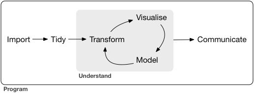
Since the beginning of this course, we have been talking about this process15 with R…but it’s not the only tool set available.
One other data science programming environment that is popular is the programming language Python16
In our first chapter, you saw the analogy of base R being like the engine and frame of a car & basic controls like the pedals and steering wheel

…the packages are the other things that enhance the car’s functions
- the body, windshield, headlights, A/C, sound system, etc

…and RStudio is the dashboard and controls

Python is a general purpose programming language, so it is like an engine.
It can power a car…or a boat, or a water pump, or …

Because Python is a general-purpose programming language, there are some key differences.
Unlike R, Python doesn’t have data analysis functions built-in.
To do data analysis in Python, you need to load the libraries (also known as the modules or packages) that are the frame, steering wheel, etc.
The libraries for this are listed below in the Resources & reference section.
For those of us who are familiar with R and RStudio, the {reticulate} package gives us an interface to add Python to our toolkit.

The reticulate package provides a comprehensive set of tools for interoperability between Python and R. The package includes facilities for:
Calling Python from R in a variety of ways including R Markdown, sourcing Python scripts, importing Python modules, and using Python interactively within an R session.
Translation between R and Python objects (for example, between R and Pandas data frames, or between R matrices and NumPy arrays).
Flexible binding to different versions of Python including virtual environments and Conda environments.
Reticulate embeds a Python session within your R session, enabling seamless, high-performance interoperability. If you are an R developer that uses Python for some of your work or a member of data science team that uses both languages, reticulate can dramatically streamline your workflow!
(from the {reticulate} site)
To load reticulate:
The {reticulate} function py_config() can be used to see what version of Python is running, and other configuration details
## python:         C:/Users/User/.virtualenvs/r-reticulate/Scripts/python.exe
## libpython:      C:/Users/User/AppData/Local/r-reticulate/r-reticulate/pyenv/pyenv-win/versions/3.9.13/python39.dll
## pythonhome:     C:/Users/User/.virtualenvs/r-reticulate
## version:        3.9.13 (tags/v3.9.13:6de2ca5, May 17 2022, 16:36:42) [MSC v.1929 64 bit (AMD64)]
## Architecture:   64bit
## numpy:          C:/Users/User/.virtualenvs/r-reticulate/Lib/site-packages/numpy
## numpy_version:  2.0.2
It’s possible to run Python code chunks inside your R Markdown document.
In this chunk, we have Python code that loads the pandas module (for data wrangling) and changes the reference to pd.
At this point, you may get a warning that pandas is not installed. If that’s the case, switch to the “Terminal” tab (next to the Console) and enter the following:
python -m pip install pandas
This next chunk reads the CSV file “flights.csv” (the flights table from {nycflights13})
# read the csv file "flights.csv" and assign it to the object "flights"
flights = pd.read_csv("data/flights.csv")

# print the head (first 5 rows)
print(flights.head())
## year month day dep_time ... distance hour minute time_hour
## 0 2013 1 1 517.0 ... 1400 5 15 2013-01-01T10:00:00Z
## 1 2013 1 1 533.0 ... 1416 5 29 2013-01-01T10:00:00Z
## 2 2013 1 1 542.0 ... 1089 5 40 2013-01-01T10:00:00Z
## 3 2013 1 1 544.0 ... 1576 5 45 2013-01-01T10:00:00Z
## 4 2013 1 1 554.0 ... 762 6 0 2013-01-01T11:00:00Z
##
## [5 rows x 19 columns]Notice a couple of things:
the read function adds an index column by default; if you have a table where you have an index variable, you can specify that in the
read_csvthat index numbering starts at 0 … watch for that if you start using row references
24.3 Filter and select
It’s a big table…over 300,000 rows.
So let’s trim it down to a bite-size chunk, and create a new Python data frame, flights_SEA:
# python chunk

# filter so that flights contains just those that are going to the
# Seattle-Tacoma airport SEA
flights_SEA = flights[flights['dest'] == "SEA"]

# select the carrier, departure delay, and arrival delay columns
flights_SEA = flights_SEA[['carrier', 'dep_delay', 'arr_delay']]

# drop the NAs
flights_SEA = flights_SEA.dropna()

# print the remainer
print(flights_SEA)
## carrier dep_delay arr_delay
## 78 AS -1.0 -10.0
## 93 DL 13.0 3.0
## 165 UA 6.0 -25.0
## 401 UA -1.0 -6.0
## 404 B6 26.0 26.0
## ... ... ... ...
## 336585 DL -1.0 10.0
## 336586 AS -6.0 5.0
## 336587 B6 30.0 35.0
## 336652 AA 4.0 -14.0
## 336685 UA 33.0 40.0
##
## [3885 rows x 3 columns]24.4 Detour: running a Python script inside your RStudio
The chunks above are defined {python} chunks.
If we have that code in a Python script “.py” file, we can run the same code inside an R chunk.
The original .py file “py_code.py” has the following:
# this wrangles the nyc13flights data using pandas

import pandas as pd
flights = pd.read_csv("data/flights.csv")
flights_SEA = flights[flights['dest'] == "SEA"]
flights_SEA = flights_SEA[['carrier', 'dep_delay', 'arr_delay']]
flights_SEA = flights_SEA.dropna()
print(flights_SEA.head())
This R chunk uses the {reticulate} function source_python() to call that file:
# r chunk that calls a Python script file

source_python("py_code.py")
## carrier dep_delay arr_delay
## 78 AS -1.0 -10.0
## 93 DL 13.0 3.0
## 165 UA 6.0 -25.0
## 401 UA -1.0 -6.0
## 404 B6 26.0 26.024.5 Calculating summary statistics
Count the number of flights to Seattle by airline: uses groupby() and size()
## carrier
## AA     360
## AS     709
## B6     513
## DL    1202
## UA    1101
## dtype: int64- the “dtype” indicates the data type, and “int64” is a 64-bit integer
Calculate the mean of departure delay, and the median of arrival delay.
## np.float64(10.6)## np.float64(-11.0)Another way to go about it would be to select the column as a new object, then calculate.
## np.float64(10.6)pandas also has a describe function that produces many summary stats:
##          dep_delay    arr_delay
## count  3885.000000  3885.000000
## mean     10.600000    -1.099099
## std      35.169665    41.933137
## min     -21.000000   -75.000000
## 25%      -4.000000   -24.000000
## 50%      -1.000000   -11.000000
## 75%       8.000000     9.000000
## max     504.000000   444.000000
24.6 Grouping
It’s possible to calculate summary statistics by a variable through the groupby function.
Here we calculate the mean delays for each airline.
##          dep_delay  arr_delay
## carrier
## AA       10.100000  -1.475000
## AS        5.830748  -9.930889
## B6       11.592593   7.721248
## DL        6.982529  -5.886023
## UA       17.321526   5.827430
The same, but with median.
##          dep_delay  arr_delay
## carrier
## AA            -2.0       -9.5
## AS            -3.0      -17.0
## B6            -1.0       -4.0
## DL            -1.0      -13.0
## UA             2.0       -5.0
24.7 Pivoting
In pandas, the reshaping functions to pivot are:
longer is
meltwider is
pivot_table
To create a longer shape:
# Python chunk

df_melted = pd.melt(flights_SEA, id_vars=["carrier"], value_vars=["dep_delay", "arr_delay"], value_name="delay.time")

print(df_melted)
## carrier variable delay.time
## 0 AS dep_delay -1.0
## 1 DL dep_delay 13.0
## 2 UA dep_delay 6.0
## 3 UA dep_delay -1.0
## 4 B6 dep_delay 26.0
## ... ... ... ...
## 7765 DL arr_delay 10.0
## 7766 AS arr_delay 5.0
## 7767 B6 arr_delay 35.0
## 7768 AA arr_delay -14.0
## 7769 UA arr_delay 40.0
##
## [7770 rows x 3 columns]The pivot_table function gives another way to calculate grouped statistics. The index variable works in the same way as groupby.
# Python chunk

df_pivot = df_melted.pivot_table(index=["carrier"], columns =["variable"], values =["delay.time"])

print(df_pivot)
## delay.time
## variable arr_delay dep_delay
## carrier
## AA -1.475000 10.100000
## AS -9.930889 5.830748
## B6 7.721248 11.592593
## DL -5.886023 6.982529
## UA 5.827430 17.321526Note that the default statistic here is the mean. We can also specify a different one using the aggfunc function:
# Python chunk

df_pivot = df_melted.pivot_table(index=["carrier"], values =["delay.time"], columns =["variable"], aggfunc='median')

print(df_pivot)
## delay.time
## variable arr_delay dep_delay
## carrier
## AA -9.5 -2.0
## AS -17.0 -3.0
## B6 -4.0 -1.0
## DL -13.0 -1.0
## UA -5.0 2.0Or we can get carried away and have multiple measures:
# Python chunk

df_pivot = df_melted.pivot_table(index=["carrier"], values =["delay.time"], columns =["variable"], aggfunc=['mean', 'median'])

print(df_pivot)
## mean median
## delay.time delay.time
## variable arr_delay dep_delay arr_delay dep_delay
## carrier
## AA -1.475000 10.100000 -9.5 -2.0
## AS -9.930889 5.830748 -17.0 -3.0
## B6 7.721248 11.592593 -4.0 -1.0
## DL -5.886023 6.982529 -13.0 -1.0
## UA 5.827430 17.321526 -5.0 2.0Pandas Pivot Table Explained, Chris Moffitt
3 Examples Using Pivot Table in Pandas (uses the gapminder table as the example)
24.8 Using Python objects in R
Assign the Python data frame “flights” created above to an R object. Some things to note:
the syntax for this is to put
py$ahead of the Python object namethis is inside an R chunk
we will now have identical data frame objects in both our Python and R environments
# r chunk

flights_SEA <- py$flights_SEA

# display
head(flights_SEA)
## carrier dep_delay arr_delay
## 78 AS -1 -10
## 93 DL 13 3
## 165 UA 6 -25
## 401 UA -1 -6
## 404 B6 26 26
## 608 UA 1 -1924.8.1 Using a Python data frame in an R {ggplot2}
library(ggplot2)

ggplot(py$flights_SEA, aes(carrier, arr_delay)) +
  geom_point()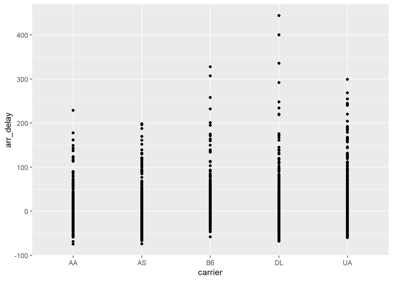
24.9 Resources & reference
24.9.1 Python as data analysis tool
There are a number of good introductory resources for using Python in data science. Here’s a short list; unfortunately, there’s not as much freely available content in the Python ecosystem:17
24.9.1.1 text books
Wes McKinney, [Python for Data Analysis]—McKinney is the lead developer behind the pandas library
Nailong Zhang, [A Tour of Data Science: Learn R and Python in Parallel], 2021
this text book has a side-by-side comparison of R and Python code to achieve the same result, including a chapter on linear regression modeling
Jake VanderPlas, Python Data Science Handbook: Essential Tools for Working with Data, 2016
- online version: https://jakevdp.github.io/PythonDataScienceHandbook/
Allen B. Downey, Elements of Data Science, 2020
Joel Grus, Data Science from Scratch: First Principles with Python (2nd edition), 2019
24.9.2 Other resources
I’ve been compiling a list of other resources that I used to understand how to tackle data science problems in Python. While the basic “this is how Python works / is different than R” things remain relevant, some of the other materials may be outdated. I’ll leave them here, should you wish to review them:
24.9.4 SciPy
(https://www.scipy.org/) – [SciPy (pronounced “Sigh Pie”) is a Python-based ecosystem of open-source software for mathematics, science, and engineering.]
The core packages include:
24.9.4.1 Pandas
pandas – data structures and analysis
10 minutes to pandas – “a short introduction to pandas, geared mainly for new users.”
data wrangling with pandas – cheat sheet
Pandas Pivot Table Explained, Chris Moffitt
3 Examples Using Pivot Table in Pandas (uses the gapminder table as the example)
“A Quick Introduction to the “Pandas” Python Library” – Adi Bronshtein, 2017-04-17
24.9.4.3 NumPy
NumPy – “the fundamental package for scientific computing with Python”
24.9.4.4 other Python data analysis modules
ggplot from ŷhat – “ggplot is a plotting system for Python based on R’s ggplot2 and the Grammar of Graphics. It is built for making profressional looking, plots quickly with minimal code.”
24.9.4.5 Jupyter notebook
First Python Notebook – a step-by-step guide to analyzing data with Python and the Jupyter notebook.
24.9.5 Calling R from Python
In our examples above, we used Python inside RStudio. An interesting recent development is that if you are working strictly in Python, you can now call all of your favourite R packages. This means that “Pythonistas can take advantage of the great work already done by the R community.”
This article walks though some examples of how Python users can access R packages:
- Isabella Velásquez, “Calling R From Python with rpy2” (2022-05-25)

-30-