6 R objects & variable types
6.1 Examining the data
R and other programming tools handle data files differently than other data analysis tools you may be familiar with, such as Excel or Google Sheets. There are two important differences:
1. How the data are accessed
The first vital difference is that in a tool like Excel, when we open the file, any changes that are made (by us or automatically by Excel) will be preserved when we save the file. This might be changes in the values, any formulas we enter into the cells, or formatting changes we make.
When we read a data file into R, we are not opening the file, and the original file is unchanged. Instead, R captures the values of the data that is stored in the file, and those values are then in the R environment—saved temporarily in the computer’s memory.
Let’s think about the words used: we open a file in Excel, but we read a file into our R environment.
2. How the data are displayed
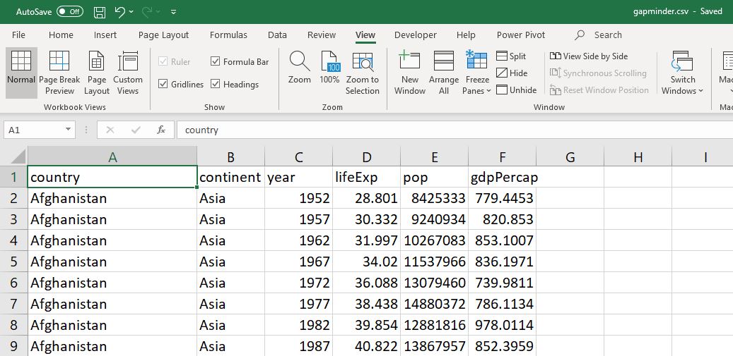
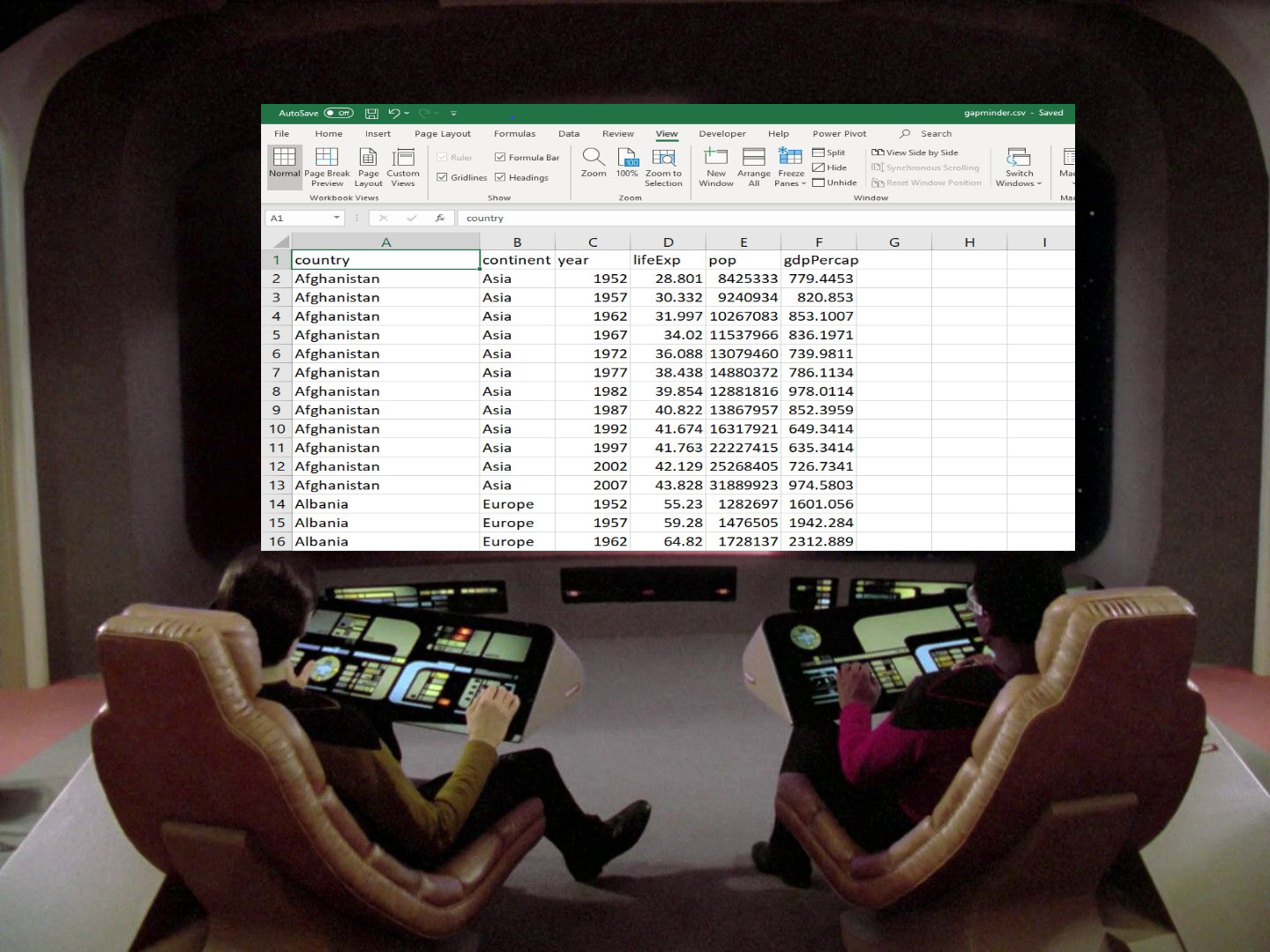
The second difference is that when we open a dataframe using a spreadsheet or other data analysis tool, we immediately see the data. In Excel, the Gapminder dataset looks like this:
Like the crew of the Enterprise, we get the data “On screen!” so we can visually investigate it.
6.1.1 Looking at data
In R, when we load a dataframe:
we assign it to an object
and that object shows up in our environment pane.
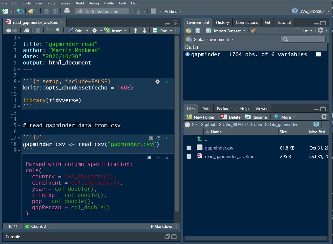
This is a different view of the universe.
In R, there are a few options for visually scanning your data:
| function | description |
|---|---|
| Content: | |
head() |
shows the first rows; the default is 6 |
tail() |
shows the last rows; the default is 6 |
view() or View()
|
display in tab |
In addition to visually inspecting the data, there are also other functions to understand a dataframe:
| function | description |
|---|---|
| Size: | |
dim() |
returns a vector with the number of rows as the first element, and the number of columns as the second element (the dimensions of the object) |
nrow() |
returns the number of rows |
ncol() |
returns the number of columns |
Functions to understand the contents of your dataframe:
| function | description |
|---|---|
| Names: | |
names() |
returns the column names (synonym of colnames() for data.frame objects) |
| Summary: | |
ls() |
returns the names in a specified environment or object |
str() |
structure of the object and information about the class, length and content of each column |
ls.str() |
combines ls() and str()
|
summary() |
summary statistics for each column |
glimpse() |
returns the number of columns and rows of the tibble, the names and class of each column, and previews as many values will fit on the screen. Unlike the other inspecting functions listed above, glimpse() is not a “base R” function so you need to have the dplyr or tibble packages loaded to be able to execute it. |
Note: most of these functions are “generic.” They can be used on other types of objects besides dataframes or tibbles.
6.2 Variable types
In R (as with other programming languages), data is stored as different variable types. In a spreadsheet program like Excel this is obscured from the user, but in R it’s explicit, and in many contexts, it matters.
int stands for integers.
dbl stands for doubles, or real numbers.
chr stands for character vectors, or strings.
date stands for dates.
dttm stands for date-times (a date + a time).
fctr stands for factors, which R uses to represent categorical variables with fixed possible values.
lgl stands for logical, vectors that contain only TRUE or FALSE.
6.3 Missing values
6.3.1 Readings
J.D. Long and Paul Teetor, R Cookbook (2nd ed.)
It is common that there are missing values in a dataset, and many reasons why this might occur. These missing values are usually represented in R as NA values (which is different than a zero or a blank cell)—these are explicitly missing values.
- they can be included as any type: e.g. numeric or character
Missing values are contagious
- an
NAin the input will return anNAin the output
6.3.2 Functions for missing values
Dealing with those pesky NA values
| function | action |
|---|---|
na.rm = TRUE |
remove NA values when running function |
is.na(x) |
returns TRUE or FALSE for each value in x
|
anyNA(x) |
returns a single TRUE or FALSE |
6.3.3 A short example
Here are three examples of what happens when NA values are part of your calculation.
Add a numeric value to an NA:
1 + NA## [1] NAAdding 1 to every item in a numeric list that includes an NA:
num_list <- c(1, 2, NA, 4, 5)
1 + num_list
## [1] 2 3 NA 5 6Calculating the mean of a numeric list that includes an NA:
mean(num_list)## [1] NA6.3.4 Functions for dealing with NA values
The functions is.na and anyNA(x) are logical—they will return a “TRUE” or “FALSE” value.
What does is.na(x) return?
## [1] FALSE TRUE FALSEThere are three values in num_list, so three tests—only the second one is NA.
What about anyNA(x)?
anyNA(num_list)## [1] TRUEOne of the three values in num_list is NA, so only one “TRUE” is returned.
What if we put an exclamation mark—the “not” symbol—in front of is.na()? How does it differ from is.na()?
!is.na(num_list)## [1] TRUE FALSE TRUEThe “NA” value in our list of numbers will cause a function like sum() to return an “NA” result. Use na.rm as an argument within the sum() function to calculate the sum of num_list:
# example
sum(num_list)
## [1] NA
# answer
sum(num_list, na.rm = TRUE)
## [1] 4