19 Exporting data & graphics

19.1 Saving data

R provides a variety of options for saving dataframes that have been created. For these examples, we will look at CSV and Excel files, but there are many other options.

19.1.1 Writing a CSV file

Write the Canada records from gapminder as a CSV file. This example uses the write_csv() function that is within the {readr} package.

• “Write a data frame to a delimited file”, from the {readr} package site

library(readr)
library(gapminder)

Filter so that only the records for Canada are included; assign to new object “gapminder_canada”

gapminder_canada <- gapminder |> 
  filter(country == "Canada")

Write the dataframe object as a csv file.

write_csv(gapminder_canada, "gm_canada.csv")

19.2 Writing an Excel file

{openxlsx}: Read, Write and Edit xlsx Files

• CRAN https://cran.r-project.org/web/packages/openxlsx/index.html

• package reference page: https://ycphs.github.io/openxlsx/

From the Introduction article at the package reference: https://ycphs.github.io/openxlsx/articles/Introduction.html

19.3 Saving graphs

ggsave() (one of the functions in {ggplot2})

https://ggplot2.tidyverse.org/reference/ggsave.html

Let’s make a plot of life expectancy changes in Canada, using the dataframe we made above:

plot_gm_canada <- ggplot(gapminder_canada, aes(x = year, y = lifeExp)) +
  geom_line()

plot_gm_canada

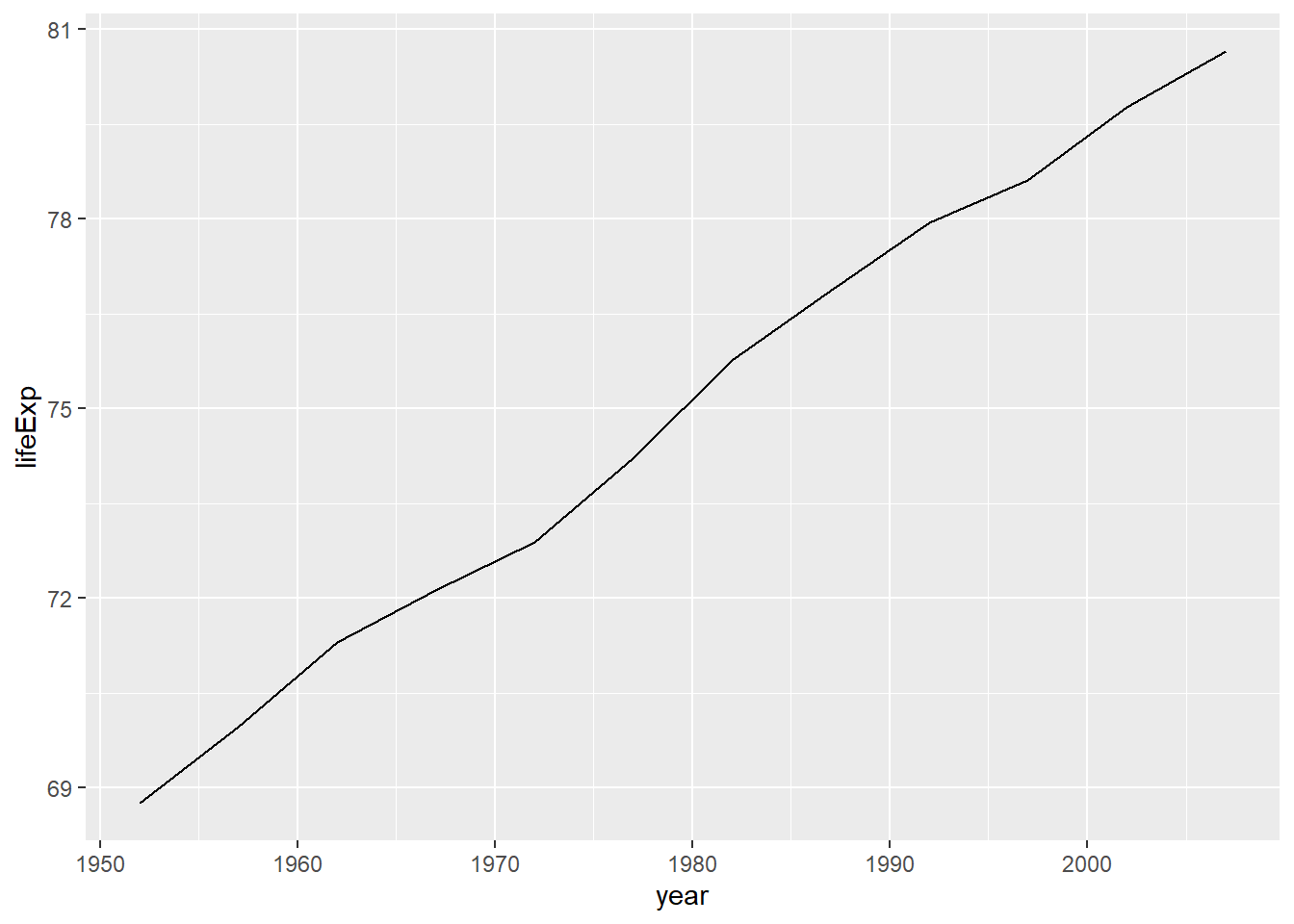
To save this plot as a separate file, we can use the ggsave() function. Note that in this example, the image hasn’t been saved into our environment as a plot object–the ggsave() function will save the last object that was created. In this version, we save the previously created plot as a png file.

ggsave("gapminder_canada_lifeexp.png")

The function has arguments that you might find useful:

• specify the file type,

• specify an object, and

• the change the dimensions to suit your purpose and data:

ggsave("gapminder_canada_lifeexp.jpg", 
  plot_gm_canada, 
  width = 9, height = 6)