Chapter 24: ANOVA

Sample from more than two normal distribution.

Motivating Scenario:
Imagine you’re interested in comparing the effectiveness of multiple treatments, observing the average heights of several plant species, or analyzing test scores across several student groups exposed to different study methods. In each of these cases, we have more than two samples, and we want to determine if there are meaningful differences among their means. While a two-sample t-test can compare two groups, comparing more than two groups would require multiple t-tests, which increases the likelihood of a false positive result due to the multiple testing problem. ANOVA allows us to evaluate whether there are significant differences among the means of multiple groups simultaneously, without increasing our chance of error.

Learning Goals: By the end of this chapter, you should be able to:

• Explain the concept of the multiple testing problem.
  
• Describe how ANOVA addresses the multiple testing problem.
  
• Identify and interpret different “sums of squares” visually and mathematically.
  
• Calculate an F-statistic and relate it to the sampling distribution.
  
• Conduct appropriate post-hoc tests for further analysis.

ANOVA Setup

We often have more than two groups to compare. For example, instead of just testing whether a fertilizer is better than a control, we might want to examine how several different fertilizers affect plant growth.

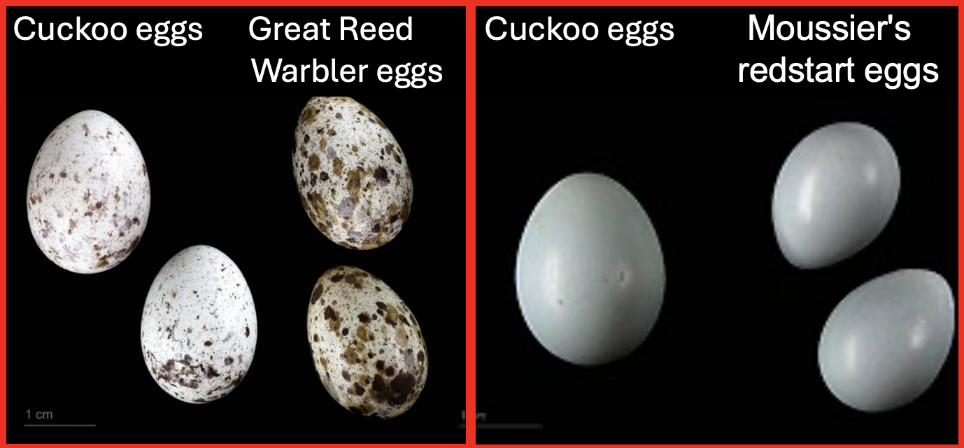
Figure 1: Eggs of the common european cuckoo next to those of its unsuspecting hosts*. Image from wikipedia.

In the extended example for this chapter, we investigate whether the size of cuckoo eggs differ across six different hosts. Remember the cuckoo’s are “brood parasites” they dump their eggs in nests of other species and hope that those thers will care for them.

The data are plotted below:

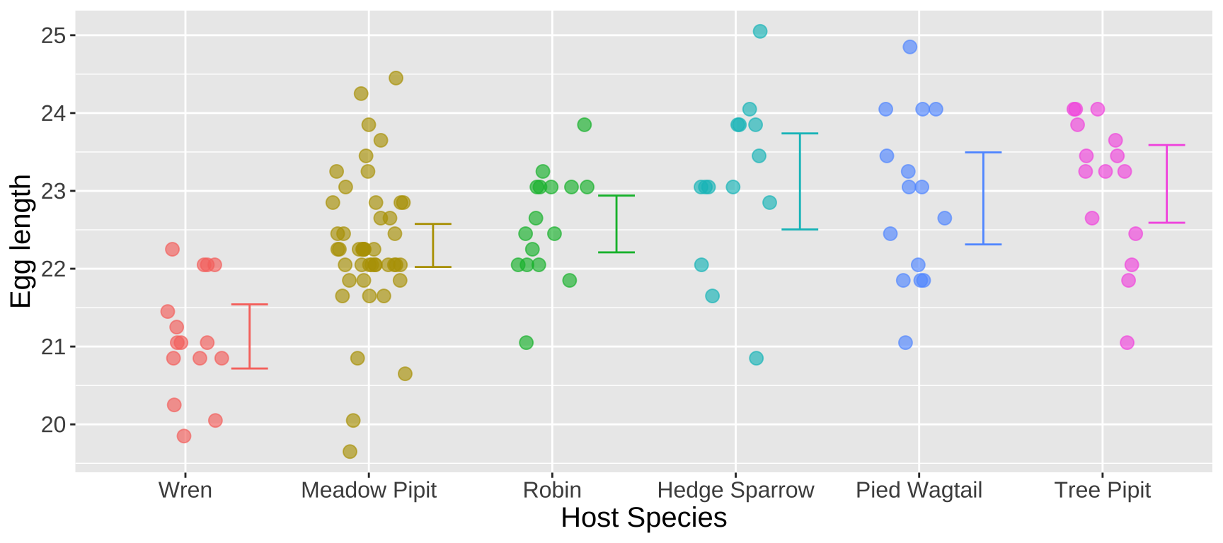
Figure 2: Distribution of egg lengths across different host species. The error bars represent the 95 percent confidence intervals within each species. Data are available here. Code is available here.

Why Not Just Perform All Pairwise t-Tests?

One possible approach is to compare all pairs of host species using t-tests. With six host species, there are \(\binom{6}{2} = 15\) possible pairwise comparisons. Below, I perform these pairwise tests but this is incorrect:

# Running pairwise t-tests between each combination of host species
dplyr::filter(cuckoo_eggs, host_species %in% c("Wren", "Meadow Pipit")) %>%
  t.test(egg_length ~ host_species, var.equal = TRUE, data = .)

dplyr::filter(cuckoo_eggs, host_species %in% c("Wren", "Robin")) %>%
  t.test(egg_length ~ host_species, var.equal = TRUE, data = .)

# (continue similar pairwise comparisons for all species pairs)

# A tibble: 15 × 5
   comp                          estimate       t    df     p.value
   <chr>                            <dbl>   <dbl> <dbl>       <dbl>
 1 Wren vs Meadow Pipit           -1.17   -4.45      58 0.0000396  
 2 Wren vs Robin                  -1.45   -5.63      29 0.00000438 
 3 Wren vs Hedge Sparrow          -1.99   -5.86      27 0.00000308 
 4 Wren vs Pied Wagtail           -1.77   -5.28      28 0.0000130  
 5 Wren vs Tree Pipit             -1.96   -6.50      28 0.000000487
 6 Meadow Pipit vs Robin          -0.276  -1.09      59 0.278      
 7 Meadow Pipit vs Hedge Sparrow  -0.823  -2.81      57 0.00677    
 8 Meadow Pipit vs Pied Wagtail   -0.604  -2.12      58 0.0387     
 9 Meadow Pipit vs Tree Pipit     -0.791  -2.90      58 0.00531    
10 Robin vs Hedge Sparrow         -0.546  -1.69      28 0.102      
11 Robin vs Pied Wagtail          -0.328  -1.03      29 0.313      
12 Robin vs Tree Pipit            -0.515  -1.80      29 0.0825     
13 Hedge Sparrow vs Pied Wagtail   0.218   0.549     27 0.587      
14 Hedge Sparrow vs Tree Pipit     0.0314  0.0858    27 0.932      
15 Pied Wagtail vs Tree Pipit     -0.187  -0.517     28 0.609      

This approach is problematic because, with 15 comparisons, we are likely to reject at least one true null hypothesis simply by chance. According to the multiplication rule from the probability chapter, the probability of failing to reject a true null hypothesis in all 15 comparisons with \(\alpha = 0.05\) is:

\[ (1 - 0.05)^{15} = 0.463 \]

Thus, the probability of rejecting at least one true null hypothesis is:

\[ 1 - 0.463 = 0.537 \]

This means there is a 53.7% chance of rejecting at least one true null hypothesis, even when all the null hypotheses are true, leading to a high risk of false positives.

The Problem of Multiple Testing

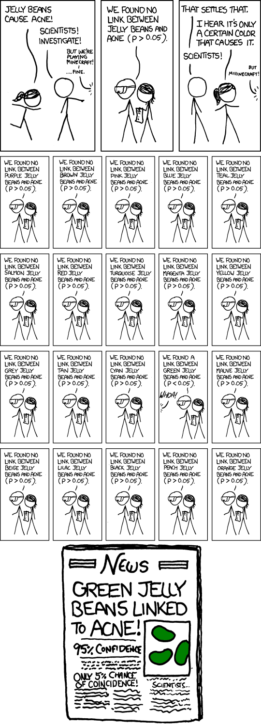
Figure 3: The multiple testing problem according to xkcd.

This classic xkcd comic (Figure 3) illustrates the problem of multiple testing. As we perform more tests, we increase the likelihood of finding a significant result by chance, even if none truly exist. When testing differences between groups, the number of pairwise comparisons increases rapidly as the number of groups grows, and subsequently the probability of at least one false positive drastically increases with the number of groups (Figure 4). How quickly? Let’s revisit the binomial coefficient formula, where \(k = 2\) (since we’re comparing pairs), and \(n\) is the number of groups:

\[ \binom{n}{2} = \frac{n(n-1)}{2} \]

So, for example, with \(n = 15\) groups, we would have 105 pairwise comparisons. The probability of rejecting at least one true null hypothesis becomes essentially guaranteed (\(1 - (1 - 0.05)^{105}= 0.9954\)).

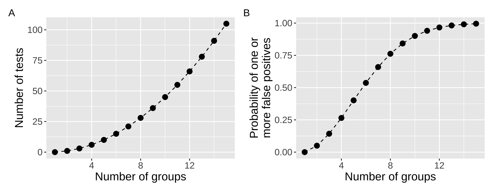
Figure 4: (A) The number of pairwise tests increases rapidly with the number of groups. (B) This essentially gauruntees a false positive with ten or more groups.

The ANOVA’s solution to the multiple testing problem

Instead of testing each combination of groups, the ANOVA poses a different null hypothesis. The ANOVA tests the null hypothesis that all samples come from the same statistical population.

ANOVA hypotheses

• \(H_0\): All samples come from the same (statistical) population. Practically, this says that all groups have the same mean.
  
• \(H_A\): Not all samples come from the same (statistical) population. Practically this says that not all groups have the same mean.

The ANOVA makes this null by some algebraic rearrangement of the sampling distribution. That is, the ANOVA tests the null hypothesis that all groups come from the same (statistical) population based on the expected variance of estimates from the sampling distribution!!

Mathemagic of the ANOVA

Recall that the standard error of the mean (\(\sigma_{\overline{Y}}\)) of a sample of size \(n\) from a normal sampling distribution is the standard deviation divided by the square root of the sample size: \(\sigma_{\overline{Y}} = \frac{\sigma}{\sqrt{n}}\).

With some algebra (squaring both sides and multiplying both side by n), we see that the sample size times the variance among groups \(n \times \sigma_{\overline{Y}}^2\) equals the variance within groups \(\sigma^2\) (Equation (1)).

\[\begin{equation} \begin{split} \sigma_{\overline{Y}} = \sigma / \sqrt{n} \\ \sigma_{\overline{Y}}^2 = \sigma^2 / n \\ n \times \sigma_{\overline{Y}}^2 = \sigma^2 \end{split} \tag{1} \end{equation}\]

• So, if all groups come from the same population (i.e. under the null hypothesis), \(n \times \sigma_{\overline{Y}}^2\) will equal the variance within groups \(\sigma^2\).

• If all groups do not come from the same population (i.e. under the alternative hypothesis), \(n \times \sigma_{\overline{Y}}^2\) will exceed the variance within groups \(\sigma^2\).

Parameters and estimates in an ANOVA

So we can turn these ideas into parameters to estimate.

Source	Parameter	Estimate	Notation
Among Groups	\(n \times \sigma_Y^2\)	Mean squares model	\(\text{MS}_\text{model}\)
Within Groups	\(\sigma^2_Y\)	Mean squares error	\(\text{MS}_\text{error}\)
Total	\(n \times \sigma_Y^2 + \sigma^2_Y\)	Mean squares total	\(MS_{total}\)

So with this new math and algebra we can restate our null and alternative hypotheses for an ANOVA

• \(H_0\): Mean squares model is not greater than mean squares error (i.e. among group variance equals zero).

• \(H_A\): Mean squares model is greater than mean squares error (i.e. among group variance is not zero).

I call \(n \times \sigma_Y^2\) mean squares model. A more common name for this is mean squares group. I call this mean squares model to emphasize that this is the same calculation we will do for all linear models.

Concepts and calculations for an ANOVA

ANOVA partitions variance

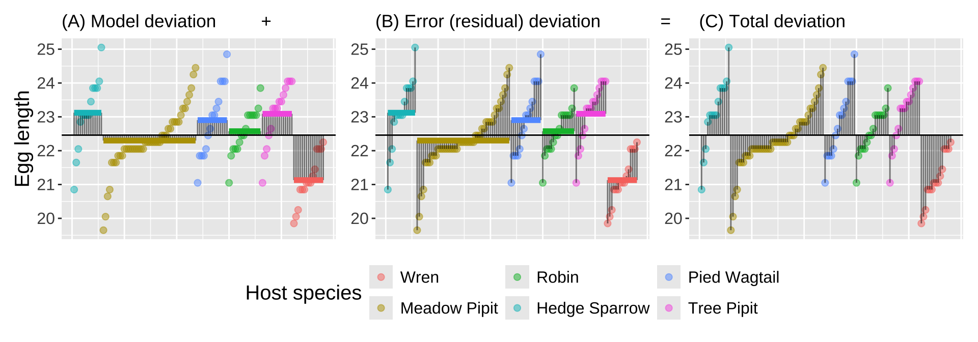
Figure 5: Partitioning deviations in an ANOVA. A Shows the difference between each observation, \(Y_i\), and the grand mean, \(\overline{\overline{Y}}\). This is the basis for calculating \(MS_{total}\). B Shows the difference between each predicted value \(\widehat{Y_i}\) and the grand mean, \(\overline{\overline{Y}}\). This is the basis for calculating \(MS_{model}\). C Shows the difference between each observation, \(Y_i\), and its predicted value \(\widehat{Y_i}\). This is the basis for calculating \(MS_{error}\).

Figure 5, really helps me understand what we are doing in ANOVA – separate the sum of the variability among (a), and within (b) groups to think about all variability in our data (c). To do this, we square the length of each line in Figure 5 and sum them. As we’ve seen before, these sums are called the “sums of squares.” Specifically:

• \(\text{SS}_\text{Model}\) represents the squared difference between the predicted value for each individual (\(\hat{x}_i\), i.e., the group mean) and the grand mean (\(\bar{x}\)), summed across all individuals: \(\text{SS}_\text{Model} = \sum(\hat{x_i} - \bar{x})^2\).

• \(\text{SS}_\text{Error}\) is the squared difference between each individual value (\(x_i\)) and its predicted value (\(\hat{x}_i\), i.e., the group mean), summed across all individuals: \(\text{SS}_\text{Error} = \sum(x_i - \hat{x}_i)^2\).

• \(\text{SS}_\text{Total}\) is calculated as the squared difference between each individual value (\(x_i\)) and the grand mean (\(\bar{x}\)), summed across all individuals: \(\text{SS}_\text{Total} = \sum(x_i - \bar{x})^2\).

Here, I introduce the augment() function from the broom package as a convenient way to calculate these components. augment() takes a linear model object as input and returns additional information about each data point, along with the original data, including:

• .fitted: The predicted value from the model.
• .resid: The residual, or the difference between the individual values and their predicted values.

cuckoo_lm <- lm(egg_length ~ host_species, data = cuckoo_eggs)
augment(cuckoo_lm)

# A tibble: 120 × 8
   egg_length host_species  .fitted  .resid   .hat .sigma   .cooksd
        <dbl> <fct>           <dbl>   <dbl>  <dbl>  <dbl>     <dbl>
 1       20.8 Hedge Sparrow    23.1 -2.27   0.0714  0.886 0.0862   
 2       21.6 Hedge Sparrow    23.1 -1.47   0.0714  0.902 0.0362   
 3       22.0 Hedge Sparrow    23.1 -1.07   0.0714  0.907 0.0192   
 4       22.8 Hedge Sparrow    23.1 -0.271  0.0714  0.913 0.00123  
 5       23.0 Hedge Sparrow    23.1 -0.0714 0.0714  0.913 0.0000852
 6       23.0 Hedge Sparrow    23.1 -0.0714 0.0714  0.913 0.0000852
 7       23.0 Hedge Sparrow    23.1 -0.0714 0.0714  0.913 0.0000852
 8       23.0 Hedge Sparrow    23.1 -0.0714 0.0714  0.913 0.0000852
 9       23.4 Hedge Sparrow    23.1  0.329  0.0714  0.913 0.00180  
10       23.8 Hedge Sparrow    23.1  0.729  0.0714  0.910 0.00886  
# ℹ 110 more rows
# ℹ 1 more variable: .std.resid <dbl>

ss_calcs <- augment(cuckoo_lm) %>%
    mutate(grand_mean = mean(egg_length)) %>%
    mutate(sqrd_total = (egg_length  - grand_mean)^2,
           sqrd_model = (.fitted - grand_mean)^2,
           sqrd_error = (egg_length  - .fitted)^2)

# now lets look at these components 
ss_calcs %>%
  select(egg_length, .fitted, .resid, sqrd_total, sqrd_model, sqrd_error)    

# A tibble: 120 × 6
   egg_length .fitted  .resid sqrd_total sqrd_model sqrd_error
        <dbl>   <dbl>   <dbl>      <dbl>      <dbl>      <dbl>
 1       20.8    23.1 -2.27        2.59       0.437    5.16   
 2       21.6    23.1 -1.47        0.656      0.437    2.17   
 3       22.0    23.1 -1.07        0.168      0.437    1.15   
 4       22.8    23.1 -0.271       0.152      0.437    0.0737 
 5       23.0    23.1 -0.0714      0.348      0.437    0.00510
 6       23.0    23.1 -0.0714      0.348      0.437    0.00510
 7       23.0    23.1 -0.0714      0.348      0.437    0.00510
 8       23.0    23.1 -0.0714      0.348      0.437    0.00510
 9       23.4    23.1  0.329       0.980      0.437    0.108  
10       23.8    23.1  0.729       1.93       0.437    0.531  
# ℹ 110 more rows

sums_of_squares <- ss_calcs %>%
  summarise(n_groups = n_distinct(host_species) ,
            n        = n(),
            ss_total = sum(sqrd_total),
            ss_model = sum(sqrd_model),
            ss_error = sum(sqrd_error))                                                                         ;                                                                                       kable(sums_of_squares, digits = 2)

n_groups	n	ss_total	ss_model	ss_error
6	120	137.19	42.94	94.25

\(r^2 = \frac{\text{SS}_\text{model}}{\text{SS}_\text{total}}\) as the “proportion variance explained”

We now have a great summary of the effect size, as the proportion of variance explained by our model \(r^2 = \frac{\text{SS}_\text{model}}{\text{SS}_\text{total}}\). For the cuckoo example \(r^2 = \frac{42.94}{137.19} =0.313\). Or in R

sums_of_squares %>%
  mutate(r2 = ss_model / ss_total)                                                                                                   %>% kable(digits = 4)

n_groups	n	ss_total	ss_model	ss_error	r2
6	120	137.188	42.9397	94.2483	0.313

In this observational study, host species explains 31.3% of the variation in cuckoo egg length. This value, represented by \(R^2\), provides a measure of how well the model explains the variance in egg length specifically for this dataset.

⚠️ WARNING ⚠️ While \(R^2\) is a useful summary of the effect size within this study, it cannot be generalized beyond this specific dataset or experimental conditions. The value of \(R^2\) depends on the unique characteristics of the study sample, such as the relative representation of each host species and the specific conditions they experience. Changes in sample composition or size can significantly affect \(R^2\).

• It is incorrect to state

Host species explains 31.3% of the variance in cuckoo egg length.

• It is correct to state

Host species explains 31.3% of the variance in cuckoo egg length in this study with data from cuckoos on 15 Wrens, 45 Meadow Pipits, 16 Robins, 14 Hedge Sparrows, 15 Pied Wagtails and 15 Tree Pipits.

To understand why, consider the effect of excluding a species from the dataset. For instance, if we remove all data on wrens, our \(R^2\) value drops drastically to 12%.

cuckoo_eggs %>% 
  filter(!(host_species == "Wren")) %>%
  lm(egg_length ~ host_species, data = .) %>% 
  summary() %>% 
  glance() %>%
  pull(r.squared)

[1] 0.1272765

Similarly, adjusting the sample sizes can alter the results. For example, suppose we wanted equal representation across species and downsampled to 14 data points per host species. This change would mostly affect the Meadow Pipit, which originally had 45 observations, while other species had between 14 and 16 observations. Since downsampling introduces randomness, we replicate this process 1,000 times to estimate a range for \(R^2\), finding that it generally falls between 34% and 43.6% (the middle 95% of the replicated samples).

replicate(1000, cuckoo_eggs %>% 
    group_by(host_species) %>%
    slice_sample(n = 14, replace = FALSE) %>%
    lm(egg_length ~ host_species, data = .) %>% 
    summary() %>% 
    glance() %>%
    pull(r.squared)) %>% quantile(c(0.025, 0.975))

     2.5%     97.5% 
0.3394492 0.4310326 

F as ANOVA’s test statistic

Thus, \(R^2\) serves as a (somewhat fragile) measure of effect size. But how can we determine how likely it is that the null model would produce a result as extreme as ours? We do this by comparing the test statistic, \(F\)—the mean squares for the model (\({MS_{model}}\)) divided by the mean squares for error (\({MS_{error}}\))—to its sampling distribution under the null hypothesis.

\[F = \frac{MS_{model}}{MS_{error}}\]

Above, we introduced \({MS_{model}}\) as an estimate of the parameter \(n \times \sigma_Y^2\), and \({MS_{error}}\) as an estimate of \(\sigma_Y^2\). But how do we calculate these values? We calculate \({SS_{model}}\) and \({SS_{error}}\) and then divide each by their respective degrees of freedom.

Calculating \(\text{MS}_\text{groups}\)

The degrees of freedom for the groups is the number of groups minus one.
\[\begin{equation} \begin{split} \text{df}_\text{model} &= n_\text{groups} - 1\\ \text{MS}_\text{model} &= \frac{\text{SS}_\text{model}}{\text{df}_\text{model}} \end{split} \end{equation}\] Recall that \(\text{SS}_\text{model}=\sum_{i}(\hat{Y}_i - \bar{\bar{Y}})^2\).

Note: An alternative calculation is \(SS_{model}=\sum_{g}(n_g \times (\hat{Y}_g - \bar{\bar{Y}})^2)\), where the subscript \(g\) refers to the \(g^{th}\) group, and \(i\) refers to the \(i^{th}\) individual.

Calculating \(\text{MS}_\text{error}\)

The degrees of freedom for the error is the total sample size minus the number of groups.
\[\begin{equation} \begin{split} \text{df}_\text{error} &= n - n_\text{groups}\\ \text{MS}_\text{error} &= \frac{\text{SS}_\text{error}}{\text{df}_\text{error}} \end{split} \end{equation}\] Recall that \(\text{SS}_\text{error}=\sum_{i}(Y_i - \bar{\bar{Y}})^2\).

Note: An alternative calculation is \(\text{MS}_\text{error}=\frac{\sum_{g}(s_g^2\times (n_g-1))}{n - n_{groups}}\)

For two groups, ANOVA and two-sample t-test give equivalent results. This is because \(\text{MS}_\text{error}\) equals the pooled variance in the two-group case.

Calculating F-statistic

The F-statistic is calculated by dividing \(\text{MS}_\text{model}\) by \(\text{MS}_\text{error}\):

\(F = \frac{\text{MS}_\text{model}}{\text{MS}_\text{error}}\)

F_summary <- sums_of_squares %>%
  mutate(df_model = n_groups - 1,
         df_error = n - n_groups,
         ms_model = ss_model / df_model,
         ms_error = ss_error / df_error,
         F_val    = ms_model / ms_error) %>%
  dplyr::select(-n, -n_groups)
F_summary %>% kable(digits = 4)

ss_total	ss_model	ss_error	df_model	df_error	ms_model	ms_error	F_val
137.188	42.9397	94.2483	5	114	8.5879	0.8267	10.3877

Testing the null hypothesis that \(F=1\)

We find a p-value by looking at the proportion of F’s sampling distribution that is as or more extreme than our calculated F value. F is parameterized by two different degrees of freedom, \(df_{model}\) and \(df_{error}\) in that order. Recall that all ways to be extreme are on the right tail of the F distribution – so the alternative model is “F is greater than one”, and we need not multiply our p-value by two.

In R:

pf(q = F_val, df1 = df_model, df2 = dr_error, lower.tail = FALSE)
pf(q = 1906, df1 = 5, df2 = 114, lower.tail = FALSE).

The pf() function works like the pnorm(), pt() and pchisq() functions, as they all look for the probability that a random sample from the focal distribution will be as large as what we are asking about (if lower.tail = FALSE):

F_summary  %>%
  mutate(p_val = pf(q = F_val, df1 = df_model, df2 = df_error, lower.tail = FALSE))  %>%
  select(df_model, df_error, ms_model, ms_error, F_val, p_val)

# A tibble: 1 × 6
  df_model df_error ms_model ms_error F_val        p_val
     <dbl>    <int>    <dbl>    <dbl> <dbl>        <dbl>
1        5      114     8.59    0.827  10.4 0.0000000315

So we resoundingly reject the null model and conclude that cuckoo egg length is associated with host species. Because this was an observational study, we cannot conclude that there is a causal relationship, or that cuckoos adjust their egg size to their hosts. An experimental study would be necessary to figure that out!

Exploring F’s sampling distribution and critical values.

Play around with the values for the degrees of freedom and see how the F distribution changes.

An ANOVA in R and understanding its output

There are two ways to conduct an ANOVA in R. They give us the same answers but one or the other can be more convenient at times.

An ANOVA with lm() and anova() functions

First, we can simply take the output of our linear model, and give this to the anova() function:

anova(cuckoo_lm)

Analysis of Variance Table

Response: egg_length
              Df Sum Sq Mean Sq F value    Pr(>F)    
host_species   5 42.940  8.5879  10.388 3.152e-08 ***
Residuals    114 94.248  0.8267                      
---
Signif. codes:  0 '***' 0.001 '**' 0.01 '*' 0.05 '.' 0.1 ' ' 1

An ANOVA with the aov() and summary() functions.

We use the aov() function to conduct an ANOVA in R. This builds us an ANOVA table. We then examine significance with the summary function.

cuckoo_anova <- aov( egg_length ~ host_species, data = cuckoo_eggs)
cuckoo_anova

Call:
   aov(formula = egg_length ~ host_species, data = cuckoo_eggs)

Terms:
                host_species Residuals
Sum of Squares      42.93965  94.24835
Deg. of Freedom            5       114

Residual standard error: 0.9092524
Estimated effects may be unbalanced

summary(cuckoo_anova)

              Df Sum Sq Mean Sq F value   Pr(>F)    
host_species   5  42.94   8.588   10.39 3.15e-08 ***
Residuals    114  94.25   0.827                     
---
Signif. codes:  0 '***' 0.001 '**' 0.01 '*' 0.05 '.' 0.1 ' ' 1

We now also can also interpret the R-squared value, as …

sums_of_squares%>% 
  mutate(r2 = ss_model / ss_total)

# A tibble: 1 × 6
  n_groups     n ss_total ss_model ss_error    r2
     <int> <int>    <dbl>    <dbl>    <dbl> <dbl>
1        6   120     137.     42.9     94.2 0.313

REASSURINGLY WE KEEP FINDINGTHE SAME TEST STATISTICS AND P-VALUES.

Post-hoc tests and significance groups

So if we find that not all groups have the same mean, how do we know which means differ? The answer is in a “post-hoc test”. We do a post-hoc test if we reject the null. I first focus on “unplanned comparisons”, in which we look at all pairs of groups, with no preconception of which may differ.

Unplanned comparisons

Post-hoc test gets over the multiple comparisons problem by conditioning on there being at least one difference and numerous pairwise tests, and altering its sampling distribution accordingly. The Tukey-Kramer method, with test stat \(q = \frac{Y_i-Y_j}{SE}\), where \(SE = \sqrt{MS_{error}(\frac{1}{n_i}+ \frac{1}{n_j})}\) is one common approach to conduct unplanned post-hoc tests.

To do this in R, we pipe the output of aov to the TukeyHSD() function

cuckoo_anova  %>%
  TukeyHSD() 

contrast	estimate	conf.low	conf.high	adj.p.value
Meadow Pipit-Wren	1.1689	0.3831	1.9547	0.0005
Robin-Wren	1.4450	0.4977	2.3923	0.0003
Hedge Sparrow-Wren	1.9914	1.0120	2.9709	0.0000
Pied Wagtail-Wren	1.7733	0.8109	2.7358	0.0000
Tree Pipit-Wren	1.9600	0.9976	2.9224	0.0000
Robin-Meadow Pipit	0.2761	-0.4911	1.0433	0.9022
Hedge Sparrow-Meadow Pipit	0.8225	0.0159	1.6291	0.0429
Pied Wagtail-Meadow Pipit	0.6044	-0.1814	1.3903	0.2325
Tree Pipit-Meadow Pipit	0.7911	0.0053	1.5769	0.0475
Hedge Sparrow-Robin	0.5464	-0.4181	1.5110	0.5726
Pied Wagtail-Robin	0.3283	-0.6189	1.2756	0.9155
Tree Pipit-Robin	0.5150	-0.4323	1.4623	0.6160
Pied Wagtail-Hedge Sparrow	-0.2181	-1.1976	0.7614	0.9872
Tree Pipit-Hedge Sparrow	-0.0314	-1.0109	0.9480	1.0000
Tree Pipit-Pied Wagtail	0.1867	-0.7758	1.1491	0.9932

We find that all pairwise comparisons to Wren differ. In other words, cuckoo eggs are significantly smaller when found in Wren nests than in nests of all other host species examined.

We also observe that cuckoo eggs laid in Meadow Pipit nests are significantly smaller than those laid in Hedge Sparrow or Tree Pipit nests, but they are not significantly different from eggs in any other nests (aside from the Wren’s, discussed above).

These are the only significant pairwise differences.

If you think about this, you might find it strange… How can we conclude that eggs from Meadow Pipit and Hedge Sparrow nests come from different populations, but lack evidence for differences between Meadow Pipit and Pied Wagtail nests, and also between Hedge Sparrow and Pied Wagtail nests? There are two explanations:

• First, you’re onto something. With sufficient power, this situation would indeed seem odd. If this were a statement about the truth of these null and alternative hypotheses, this scenario wouldn’t be logically possible.
• Second, note my careful wording: I said, “We don’t have enough evidence that they come from different populations…” rather than “they come from the same population.” Remember, we don’t accept the null hypothesis; we simply fail to reject it.

Assigning significance groups

“Significance groups” are a simple way to summarize these complex relationships. Here, we assign the same letter to groups that do not significantly differ, and different letters to groups that do. In our case:

• Eggs laid in Wren nests form their own significance group, labeled a.
• Eggs laid in Meadow Pipit nests differ from Wren eggs, so we assign them to significance group b.
• Eggs laid in Hedge Sparrow and Tree Pipit nests are significantly longer than those in Meadow Pipit nests, so Hedge Sparrow and Tree Pipit belong to group c.
• All other nests differ significantly from Wren nests but not from one another, so they fall into significance groups b and c.

We typically mark significance groups on a plot like Figure 6.

significance_groups <- tibble(host_species = c("Wren","Meadow Pipit", "Robin",
                                    "Hedge Sparrow","Pied Wagtail", "Tree Pipit"),
                              sig_group = c("a","b","b,c", "c", "b,c","c"))

ggplot(cuckoo_eggs, aes(x = host_species, y = egg_length, color  = host_species))+
  geom_jitter(height = 0, width = .2, size = 3, alpha = .65, show.legend = FALSE)+
  stat_summary(fun.data = "mean_cl_normal", geom = "errorbar", width = .2,position =position_nudge(x = .35))+
  geom_label(data = significance_groups, aes(y = 26.5, label =  sig_group), size =7)+
  theme(axis.title = element_text(size = 15), axis.text = element_text(size = 12), legend.position = "NA")+
  labs(x = "Host Species", y = "Egg length")+
  coord_cartesian(ylim = c(19.5,27.5))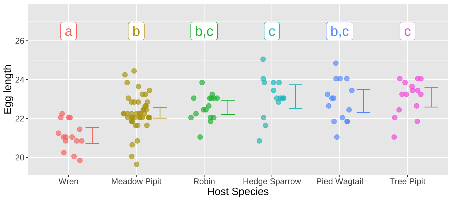

Figure 6: Figure 2… now with signigficance groups!

A wrong way to do things.

R makes it very easy to do things wrong. For example, say you ran your ANOVA on the lm() output (e.g., lm(y ~ groups) %>% anova()). This is fine and will be correct! But let’s say instead you passed your linear model results to summary(), or equivalently tidy() (as we did with the t-tests). This will give us strange answers that we don’t want. Let me show you!

cuckoo_lm %>%
  summary()

Call:
lm(formula = egg_length ~ host_species, data = cuckoo_eggs)

Residuals:
     Min       1Q   Median       3Q      Max 
-2.64889 -0.44889 -0.04889  0.55111  2.15111 

Coefficients:
                          Estimate Std. Error t value Pr(>|t|)    
(Intercept)                21.1300     0.2348  90.004  < 2e-16 ***
host_speciesMeadow Pipit    1.1689     0.2711   4.312 3.46e-05 ***
host_speciesRobin           1.4450     0.3268   4.422 2.25e-05 ***
host_speciesHedge Sparrow   1.9914     0.3379   5.894 3.91e-08 ***
host_speciesPied Wagtail    1.7733     0.3320   5.341 4.78e-07 ***
host_speciesTree Pipit      1.9600     0.3320   5.903 3.74e-08 ***
---
Signif. codes:  0 '***' 0.001 '**' 0.01 '*' 0.05 '.' 0.1 ' ' 1

Residual standard error: 0.9093 on 114 degrees of freedom
Multiple R-squared:  0.313, Adjusted R-squared:  0.2829 
F-statistic: 10.39 on 5 and 114 DF,  p-value: 3.152e-08

• Here, the (Intercept) is our reference group (in this case, Wren). The t-statistic here tests the null hypothesis that the length of cuckoo eggs laid in Wren nests is zero. This is absurd. Ignore this value and the associated p-value.

• The estimates, t-values, and p-values for all other groups describe the difference from the null hypothesis that they do not differ from the reference group. While not entirely wrong (and the estimate is key to our linear model, see below), this isn’t usually what the hypothesis test we care about, and the p-values are slightly miscalibrated.

ANOVA as a Linear Model

Earlier, I cautioned against focusing too much on the p-values for individual factors in the summary() of lm() in R. This is because:

• The (Intercept) evaluates the null hypothesis that the mean of the reference group is zero, which is often trivial.
• The estimates for each host_species level describe the difference from the reference group, rather than capturing all pairwise differences.

However, there is valuable information in this output. Most importantly, the estimates help us make predictions, and the standard errors indicate the uncertainty around each estimate.

To predict an the value of the \(i^{th}\) individual \(\hat{Y}_i\), we can use the following formula:

\[ \hat{Y}_i = a + b_1 x_{1,i} + b_2 x_{2,i} + \dots \]

where: - \(a\) is the intercept, representing the mean of the reference group, - \(b_1\), \(b_2\), etc., are the coefficients for each non-reference group, - \(x_{1,i}\), \(x_{2,i}\), etc., are binary indicators (0 or 1) that activate the respective coefficient if an observation belongs to a particular group.

This means that: - Everyone receives the intercept \(a\) (the mean of the reference group). - If an observation belongs to the first non-reference group, we add \(b_1\), and if it belongs to the second non-reference group, we add \(b_2\), and so forth.

From the summary() table above, we can then predict the outcome for any group by applying the appropriate coefficients.

• \(\hat{Y}_\text{i|Host species == Hedge} = 21.1300\).
• \(\hat{Y}_\text{i|Host species == Meadow Pipit} = 21.1300 + 1.1689 = 22.2989\).
• \(\hat{Y}_\text{i|Host species == Robin} = 21.1300 + 1.4450 = 22.575\).
  
• \(\hat{Y}_\text{i|Host species == Hedge Sparrow} = 21.1300 + 1.9914 = 23.1214\).
  
• \(\hat{Y}_\text{i|Host species == Pied Wagtail} = 21.1300 + 1.7733 = 22.9033\).
  
• \(\hat{Y}_\text{i|Host species == Tree Pipit} = 21.1300 + 1.9600 = 223.09\).

Assumptions of ANOVA

Like the two-sample t-test, ANOVA assumes:

• Independence
  
• Random sampling (no bias)
  
• Equal variance among groups (homoscedasticity)
  
• Normality within each group — or more specifically, normality of each group’s sampling distribution.

ANOVA Assumes Equal Variance Among Groups

This makes sense, as we use a mean squares error in ANOVA. In fact, the very derivation of ANOVA assumes that all groups have equal variance.

• Homoscedasticity means that the variance of residuals is independent of the predicted value. For our cuckoo eggs, we make only six predictions — one per host species group — so this essentially means we assume equal variance within each group.

cuckoo_eggs %>%
  group_by(host_species) %>%
  summarise(variance = var(egg_length)) %>%
  kable(digits = 4)

host_species	variance
Wren	0.5531
Meadow Pipit	0.8476
Robin	0.4687
Hedge Sparrow	1.1422
Pied Wagtail	1.1398
Tree Pipit	0.8126

Since all these variances are within a factor of five, we consider this a minor violation of the equal variance assumption. Like the two-sample t-test, ANOVA is robust to slight violations of equal variance among groups.

The ANOVA assumes normally distributed residuals

Note this means we assume the differences from group means are normally distributed, not that the raw data are.

As we saw for a one and two sample t-test, the ANOVA (like all linear models) is quite robust to this assumption. This is because we are actually assuming a normal sampling distribution within groups, rather than a normal distribution within groups. Still this assumption is worth checking

Let do this our self by making a qqplot and by plotting a histogram of the residuals.

qq_cuckoo <- cuckoo_eggs %>%
  ggplot(aes(sample = egg_length)) +
  geom_qq()                      +
  geom_qq_line()                  +
  facet_wrap(~ host_species, ncol = 2, scales = "free_y")+
  theme(strip.text = element_text(size = 12))


hist_cuckoo <- cuckoo_eggs %>%
  ggplot(aes(x = egg_length))+
  geom_histogram(bins = 30, color = "white")  +
  facet_wrap(~ host_species, ncol = 2, scales = "free_y")+
  theme(strip.text = element_text(size = 12))

qq_cuckoo + hist_cuckoo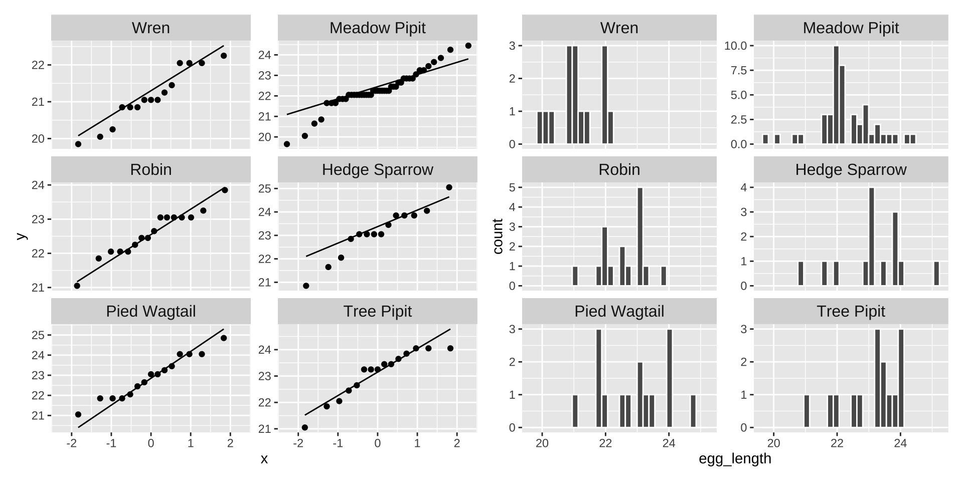

The data appear to be largely normal (except maybe the Meadow Pipit looks a bit strange). But nothing looks terrible źand I would feel comfortable assuming normality here.

Alternatives to an ANOVA

If you think data do not meet assumptions you can

• Consider this as a caveat when discussing your results, and think through how it could impact your inference.
  
• Find a more appropriate test.
  
• Write down your own likelihood function and conduct a likelihood ratio test.
  
• Permute

NOTE: Permuting DOES NOT solve the issue of unequal variance in groups. Why is that? it is because permuting will shuffle data between groups, resulting in an equal variance, so it doesnt solve this problem.

Quiz

Figure 7: Quiz on the ANOVA here

Definitions, Notation, and Equations

ANOVA (Analysis of Variance): A statistical method to test whether the means of three or more groups differ significantly. It partitions the total variance between and within groups.

Mean Squares Model (\(\text{MS}_{model}\)): The mean of the squared deviations between group means and the overall mean. Also referred to as Mean Squares Between Groups.

Mean Squares Error (\(\text{MS}_{error}\)): The mean of the squared deviations of individual observations from their group mean, representing within-group variance.

F-statistic: A ratio of variances calculated as \(\frac{\text{MS}_{model}}{\text{MS}_{error}}\), used in ANOVA to determine whether group means significantly differ. Higher values indicate greater between-group variation relative to within-group variation.

Null Hypothesis for the ANOVA (H₀): The assumption that all group means are equal, indicating no significant difference among them. Under the null \(F\) equals one. In ANOVA tests we only look at the upper tail of the F distribbtion, as it encompases all the ways that groups can differ.

Alternative Hypothesis for the ANOVA (H₁): Indicates at least one group mean differs from others.

Degrees of Freedom from the ANOVA (df): For ANOVAs, degrees of freedom are split between the model (dfₘ) and error (dfₑ). dfₘ = \(k - 1\) (number of groups minus 1) and dfₑ = \(N - k\) (total observations minus the number of groups).

R Functions for ANOVA

ANOVA Functions
lm(): Fits the ANOVA as a linear model.
anova(): Computes the ANOVA table for a linear model, showing the sums of squares, mean squares, and F-statistic.
aov(): A function designed for ANOVA calculations. It takes a model formula as input and generates an ANOVA object.

Summarizing Functions
summary(): Summarizes the ANOVA output, often used in conjunction with aov() to generate an ANOVA table,

Key Equations

1. F-statistic Formula \[ F = \frac{\text{MS}_{model}}{\text{MS}_{error}} \] where:

   • \(\text{MS}_{model} = \frac{\text{SS}_{model}}{\text{df}_{model}}\),
   • \(\text{MS}_{error} = \frac{\text{SS}_{error}}{\text{df}_{error}}\).

2. Calculating Sum of Squares for the Model (Between-Groups) \[ \text{SS}_{model} = \sum_{i=1}^{n} (\hat{Y_i} - \bar{Y})^2 = \sum_{g=1}^{k} n_g (\bar{Y}_g - \bar{Y})^2 \] where:

   • \(n_g\) is the number of observations in group \(g\),
   • \(\bar{Y}_g\) is the mean of group \(g\), This is the same as \(\hat{Y}_i\) as an individual’s predicted value is its group mean.
     
   • \(\bar{Y}\) is the overall “grand” mean.

3. Calculating Sum of Squares for Error (Within-Groups) \[ \text{SS}_{error} = \sum_{i=1}^{n} (Y_i - \hat{Y_i})^2 = \sum_{g=1}^{k} \sum_{i=1}^{n_g} (Y_{gi} - \bar{Y}_g)^2 \] where \(Y_{gi}\) is the individual observation within group \(g\).

4. Total Sum of Squares \[ \text{SS}_{total} = \text{SS}_{model} + \text{SS}_{error} = \sum_{i=1}^{n} (Y_i - \bar{Y})^2 \]