Chapter 18: Permuting II

Shuffling to test for non-random associations.

One of the most common statistical questions is, “Are these two variables associated?” For example, we might want to know if people who study more tend to get better grades. If such an association exists, especially in a randomized controlled experiment, it could suggest that studying causes better outcomes. We previously learned to quantify such associations by calculating covariance (how much x and y tend to depart from the mean in the same individual), correlation (how reliably x and y are associated), or a slope (how much y changes with x).

As we saw in the chapter on Null Hypothesis Significance Testing, frequentist statistics do not address this question directly. Instead, we approach it indirectly by asking: “Assuming there is no association between the variables, how unlikely would it be to observe an association as extreme as what we see in the data?” With this approach, we “reject the null hypothesis” of no association if the null hypothesis rarely produces such an extreme result. Conversely, we fail to reject the null if the null model frequently generates a result like the one observed.

Learning goals: In this chapter, we will revisit these summaries—quantifying uncertainty in them through bootstrapping and testing the null hypothesis of no association using permutation. We will also briefly explore interpreting standard errors (SE) and p-values from linear models in R, with a more rigorous approach to come later. Finally, we will introduce the \(\chi^2\) test, a classic parametric test for evaluating the null hypothesis of no association between categorical variables.

Review of Covariance, Correlation, and Regression

Math

Covariance is the sum of the cross products divided by the sample size minus one:

\[\begin{equation} \begin{split} Cov(X,Y) = \frac{\sum{\Big((X_i-\overline{X}) \times (Y_i-\overline{Y})\Big)}}{n-1}\\ \end{split} \tag{1} \end{equation}\]

The correlation standardizes the covariance by dividing it by the standard deviations of \(X\) and \(Y\):

\[\begin{equation} \begin{split} Cor(X,Y) = \frac{Cov(X,Y)}{s_x \times s_y}\\ \end{split} \tag{2} \end{equation}\]

Where \(s_x\) and \(s_y\) are the standard deviations of \(X\) and \(Y\) (e.g., \(\sqrt{\Sigma((x_i-\bar{x})^2)/(n-1)}\)).

Finally, the slope is the covariance divided by the variance in \(X\):

\[\begin{equation} \begin{split} b(X,Y) = \frac{Cov(X,Y)}{s^2_x}\\ \end{split} \tag{3} \end{equation}\]

Calculations in R

Let us revisit our example from our section on associations – the relationship between body mass and flipper length in our palmer penguin dataset.

ggplot(penguins, aes(x = body_mass_g, y = flipper_length_mm))+
  geom_point()+
  geom_smooth(method = 'lm')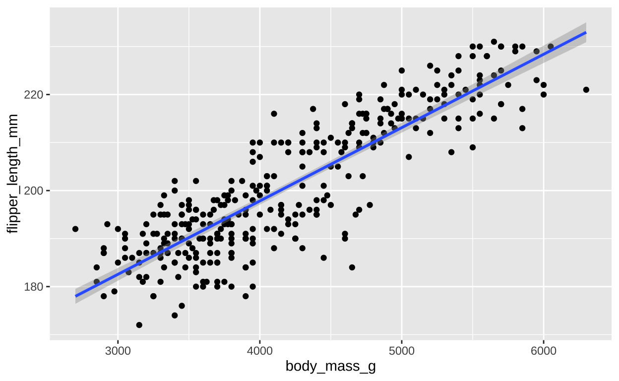

Figure 1: The relationship between body mass (x) and flipper length (y) for all samples in the Palmer Penguins dataset. The blue line represents the line of best fit, and the grey shading around it indicates the standard error (SE) of the predicted mean at each value of x.

We can calculate the covariance by explicitly writing the math out in R or by using the cov() function:

penguins %>%
  filter(!is.na(body_mass_g) & !is.na(flipper_length_mm)) %>%
  summarise(cov_penguin = cov(body_mass_g, flipper_length_mm),
            r_penguin   = cor(body_mass_g, flipper_length_mm),
            b_penguin = cov(body_mass_g, flipper_length_mm) / var(body_mass_g))

# A tibble: 1 × 3
  cov_penguin r_penguin b_penguin
        <dbl>     <dbl>     <dbl>
1       9824.     0.871    0.0153

Note that we had to calculate the slope ourselves. But R can do this too if we make a linear model:

penguins_model  <- lm(flipper_length_mm ~ body_mass_g, data = penguins)
penguins_model 

Call:
lm(formula = flipper_length_mm ~ body_mass_g, data = penguins)

Coefficients:
(Intercept)  body_mass_g  
  136.72956      0.01528  

You can see that R’s answer matches ours. We can also get more out of this model with the summary() function:

summary(penguins_model)

Call:
lm(formula = flipper_length_mm ~ body_mass_g, data = penguins)

Residuals:
     Min       1Q   Median       3Q      Max 
-23.7626  -4.9138   0.9891   5.1166  16.6392 

Coefficients:
             Estimate Std. Error t value Pr(>|t|)    
(Intercept) 1.367e+02  1.997e+00   68.47   <2e-16 ***
body_mass_g 1.528e-02  4.668e-04   32.72   <2e-16 ***
---
Signif. codes:  0 '***' 0.001 '**' 0.01 '*' 0.05 '.' 0.1 ' ' 1

Residual standard error: 6.913 on 340 degrees of freedom
  (2 observations deleted due to missingness)
Multiple R-squared:  0.759, Adjusted R-squared:  0.7583 
F-statistic:  1071 on 1 and 340 DF,  p-value: < 2.2e-16

Here we find the slope as the Estimate for body_mass_g in the table. We should feel reassured that 1.528e-02 is just another way to write 0.01528, so our answers match.

This summary of our linear model also provides other useful bits of information — including the standard error of this (and other estimates) and \(r^2\) or ‘proportion of variance explained.’ Again, we should feel good that taking the square root of \(r^2\) (reported as 0.759) gives us 0.8712 — the same number as our correlation coefficient, \(r\). Later in this term, we will engage more deeply with the lm() function and interpretations of this summary output as we delve further into linear models. For now - know that these stats make a few assumptions about the shape of our residauls that we can circumvent by bootstrapping.

Quantifying uncertainty and null hypothesis significance testing.

Estimate Uncertainty by Bootstrapping

Estimation is just the beginning of a statistical analysis. Next, we need to evaluate the uncertainty in our estimates. Recall from the previous section that we quantify uncertainty by imagining that an estimate is a sample from an unknown sampling distribution. We can measure this uncertainty through:

• Standard error (SE): The standard deviation of the sampling distribution.
  
• 95% confidence interval (95% CI): The range between the upper and lower 2.5% tails of the sampling distribution.

While we almost never know the true sampling distribution, bootstrapping —- resampling our data randomly with replacement—provides a powerful way to approximate it.

Figure 2: Resampling to stimate uncertainty in the slope. Each frame represents a new bootstrap replicate. We can see that the slope is pretty stable ranging between 0.0145 and 0.016.

boot_slope <- replicate(1000, simplify = FALSE, {
  penguins %>%
    filter(!is.na(flipper_length_mm + body_mass_g)) %>%
    slice_sample(prop = 1, replace = TRUE) %>%
    summarise(b_boot   = cov(body_mass_g, flipper_length_mm) / var(body_mass_g))}) %>% 
  bind_rows()

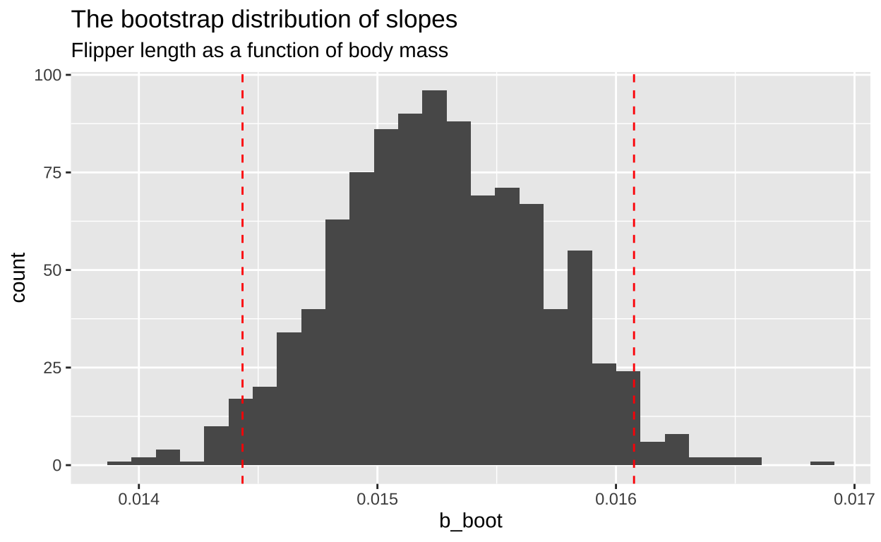
Figure 3: A histrogram showing the disitrbution of the estimated slope across one thousand bootstrap replicates. The 95 percent CI is show with dotted red lines. code here

Now that we’ve approximated the sampling distribution, we can estimate our uncertainty:

boot_slope %>%
  summarise(se=sd(b_boot), 
            lower_95_CI = quantile(b_boot, prob = 0.025),
            upper_95_CI = quantile(b_boot, prob = 0.975))

# A tibble: 1 × 3
        se lower_95_CI upper_95_CI
     <dbl>       <dbl>       <dbl>
1 0.000435      0.0144      0.0161

It’s reassuring that our estimate of the standard error is quite close to the results from the linear model summary (4.668e-04, as shown earlier).

Null Hypotehsis Significance Testing by permutation

Now we will test the null hypothesis of no slope by using permutation. To do this, we generate a null distribution by randomly reassigning body weight to different penguins and measuring how often the slope (or covariance, or correlation—all of which will yield the same p-value) from this random assignment is as extreme or more extreme than the slope we observed in the actual data.

As another visual comparison, let’s examine the slope from the actual data alongside the distribution of slopes generated from the permuted data.

perm_slope <- replicate(1000, simplify = FALSE, {
  penguins %>%
    filter(!is.na(flipper_length_mm + body_mass_g)) %>%
    mutate(perm_body_mass_g =  sample(body_mass_g, replace = FALSE)) %>%
    select(species, flipper_length_mm, perm_body_mass_g)}) %>%
  bind_rows(.id = "replicate_id") %>%
  group_by(replicate_id) %>%
  summarise(cov_perm = cov(perm_body_mass_g, flipper_length_mm),
         r_perm   = cor(perm_body_mass_g, flipper_length_mm),
         b_perm   = cov(perm_body_mass_g, flipper_length_mm) / var(perm_body_mass_g))%>%
  ungroup()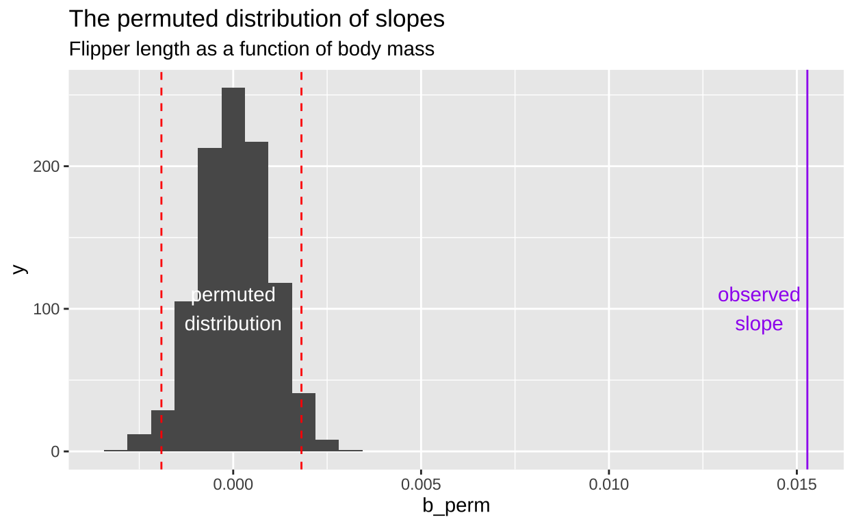

Figure 4: A histogram displaying the distribution of slopes (b_perm) generated from permuted data for the relationship between flipper length and body mass. The x-axis represents the permuted slope values, while the y-axis represents the count of each slope value. The bulk of the permuted slopes are centered around zero. Two red dashed lines represent the 2.5th and 97.5th percentiles of the permuted distribution, forming the 95 percent confidence interval. A purple vertical line on the far right marks the observed slope from the actual data, far beyond the permuted distribution, labeled observed slope. code here

The plots above show that the actual slope is significantly steeper compared to any of the one hundred permutations we visualized. This visual alone suggests that the p-value is likely much less than 0.01. To formally calculate the p-value, we would determine the proportion of permutations with a slope as extreme or more extreme than what we observed. However, in this case, it’s clear that the p-value is very low, and we would need shitloads of permutations just to find one as extreme as ours. Therefore, we can confidently reject the null hypothesis that the slope is zero and move on to a more statistically interesting example.

Comparing Slopes

Let’s say we want to determine if the slopes differ by species. This question is more interesting both biologically and statistically! For fun, let’s compare the slopes of Adelie and Chinstrap penguins:

focal_penguins <- penguins %>%
  filter(species %in% c("Adelie","Chinstrap")) %>%
  filter(!is.na(flipper_length_mm + body_mass_g)) %>%
  select(species, flipper_length_mm, body_mass_g)

gg_color_hue <- function(n) { hues = seq(15, 375, length = n + 1); hcl(h = hues, l = 65, c = 100)[1:n] }
ggplot(focal_penguins, aes(x = body_mass_g, y = flipper_length_mm, color = species)) +
  geom_point() +
  geom_smooth(method = 'lm') + 
  scale_color_manual(values = gg_color_hue(3)[1:2],            # keeping colors the same as above
                     guide = guide_legend(reverse = TRUE)) +  # swapping order in the legend
  geom_label(data = . %>%
    group_by(species) %>%
    summarise(slope = cov(body_mass_g, flipper_length_mm) / var(body_mass_g),
              slope_label = paste(unique(species), "\nslope:", round(slope, digits = 4)),
              body_mass_g = 5200,
              flipper_length_mm = max(c(as.numeric(species == "Chinstrap") * 209, 197))),
             aes(label = slope_label), size = 6) +
  coord_cartesian(xlim = c(2500, 5500)) +
  theme(legend.position = "none")

Figure 5: A plot of the relationship between body mass and flipper length. code here

We can see that the slopes appear to differ—flipper length increases faster with body mass in Chinstrap penguins compared to Adelie penguins. Before we think about swapping labels for permutation, consider what happens when we swap values—we are also moving into datasets with different means and standard deviations.

focal_penguins %>%
  group_by(species) %>%
  summarise(mean_flipper_length_mm = mean(flipper_length_mm), 
            mean_body_mass_g       = mean(body_mass_g), 
            sd_flipper_length_mm   = sd(flipper_length_mm), 
            sd_body_mass_g         = sd(body_mass_g))

# A tibble: 2 × 5
  species mean_flipper_length_mm mean_body_mass_g sd_flipper_length_mm
  <fct>                    <dbl>            <dbl>                <dbl>
1 Adelie                    190.            3701.                 6.54
2 Chinst…                   196.            3733.                 7.13
# ℹ 1 more variable: sd_body_mass_g <dbl>

So, let’s transform each data point by subtracting the species mean and dividing by the standard deviation. We will later learn that this is a common practice called a Z-transform.

Ztrans <- function(x) { (x - mean(x)) / sd(x) }  # Writing our own function to Z-transform

z_focal_penguins <- focal_penguins %>%
  group_by(species) %>%
  mutate_all(Ztrans)  # Applying the Z-transform to all variables

Figure 6: A plot of the relationship between Z-transformed body mass and flipper length. code here.

Bootstrap for Uncertainty

We observe that the difference in slopes for the Z-transformed data is 0.6416 - 0.4682 = 0.1734. Our bootstrap analysis below reveals a 95% confidence interval that ranges from slightly below zero to a little over 0.4. This means we cannot exclude zero as a plausible difference in slopes.

boot_slope_diff <- replicate(1000, simplify = FALSE,
  z_focal_penguins %>%
    group_by(species) %>%
    slice_sample(prop = 1, replace = TRUE) %>%
    summarise(slope = cov(flipper_length_mm, body_mass_g) / var(body_mass_g)) %>%
    summarise(diff_slope = diff(slope))) %>%
  bind_rows()

Figure 7: The bootstrap distribution for the difference in slopes. code here

Permute to Test the Null Hypothesis

We observed that the difference in slopes for the Z-transformed data is 0.6416 - 0.4682 = 0.1734. Our permutation test below reveals that this difference could be readily generated by a null model. This suggests we cannot exclude zero as a plausible difference in slopes.

perm_dist_z <- replicate(1000, simplify = FALSE,
  z_focal_penguins %>%
    ungroup() %>%
    mutate(species = sample(species, replace = FALSE)) %>%
    group_by(species) %>%
    summarise(slope = cov(flipper_length_mm, body_mass_g) / var(body_mass_g)) %>%
    summarise(perm_diff_slope = diff(slope))) %>%
  bind_rows()

Figure 8: The permuted distribution for the difference in slopes. The observed slope (purple) falls within 95 percent of the samples from the null distribution (shown in red). code here

The figure above is consistent with our bootstrap results— the observed difference in slopes can be easily generated by the null model. To calculate a p-value, we can determine the proportion of permutations where the absolute value of the difference in slopes exceeds the observed value.

diff_slope_obs <- z_focal_penguins %>% 
  group_by(species) %>%
  summarise(slope = cov(flipper_length_mm, body_mass_g) / var(body_mass_g)) %>% 
  summarise(diff_slope = diff(slope)) %>%
  pull()

perm_dist_z %>%
  mutate(as_or_more = abs(perm_diff_slope) >= abs(diff_slope_obs)) %>%
  summarise(p_val = mean(as.numeric(as_or_more)))

# A tibble: 1 × 1
  p_val
  <dbl>
1 0.132

Therefore, we fail to reject the null hypothesis! In the world of null hypothesis significance testing we cannot say that these species have different slopes.

Associations Between Categorical Variables

We have previously discussed that associations aren’t limited to continuous variables; we can also describe associations between categorical variables, often in the form of covariance or correlation. Let’s explore the covariance between a penguin being an “Adelie” species and its origin from “Biscoe” island.

penguins_binary <- penguins %>%
  mutate(Adelie = species == "Adelie",
         Biscoe = island == "Biscoe") %>% 
  select(species, Adelie, island, Biscoe)

We can visualize the distribution of these binary variables using a bar plot:

ggplot(penguins_binary, aes(x = Adelie, fill = Biscoe)) +
  geom_bar()

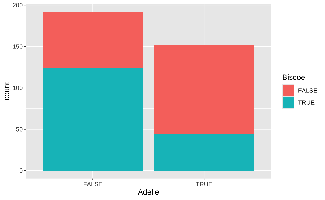
Next, we summarize the association as usual (treating TRUE as 1 and FALSE as 0):

penguins_binary %>%
  summarise(cov = cov(Adelie, Biscoe), 
            cor = cor(Adelie, Biscoe))

# A tibble: 1 × 2
      cov    cor
    <dbl>  <dbl>
1 -0.0881 -0.354

Permuting to Test the Null

To find the p-value, we can permute as usual. Here, we see that the p-value is very low (though we typically report it as less than 0.001, rather than calling it zero).

replicate(1000, simplify = FALSE,
          penguins_binary %>%
            mutate(perm_island = sample(island),
                   perm_biscoe = perm_island == "Biscoe") %>%
            summarise(cov_perm = cov(Adelie, perm_biscoe),
                      cov_obs  = cov(Adelie, Biscoe)) %>%
            mutate(as_or_more = abs(cov_perm) >= abs(cov_obs))) %>% 
  bind_rows() %>%
  summarise(p_val = mean(as_or_more))

# A tibble: 1 × 1
  p_val
  <dbl>
1     0

\(\chi^2\)

The \(\chi^2\) statistic is a widely-used summary for comparing count data across categories. To calculate \(\chi^2\), we follow these steps:

1. Find the expected number of observations for each category. (For a \(\chi^2\) contingency test, the expected value comes from the multiplication rule—the expected frequency of two independent events is the product of their probabilities.)
2. Find the difference between the observed and expected values.
3. Square that difference.
4. Divide by the expected value.
5. Sum these values across all categories.

The formula for \(\chi^2\) is:

\[\chi^2 = \Sigma \frac{(\text{observed}_i - \text{expected}_i)^2}{\text{expected}_i}\]

For a \(\chi^2\) contingency test, the expected value is calculated using the multiplication rule, where the expected frequency of two independent events is the product of their individual probabilities.

Degrees of Freedom

When calculating \(\chi^2\), we also need to consider the degrees of freedom (df). We will talk about degress of freedom more later in the term. In contingency tables, the degrees of freedom are calculated as:

\[ \text{df} = (\text{number of rows} - 1) \times (\text{number of columns} - 1) \]

This reflects the number of independent comparisons we can make, given that the total counts are fixed. In this case, since we are working with a 2x2 table (Adelie and Biscoe as binary variables), the degrees of freedom are 1.

Calculating \(\chi^2\) from the Data

Let’s calculate \(\chi^2\) for our data:

chi_cals <- penguins_binary %>%
    group_by(Adelie, Biscoe) %>%
    tally() %>%
    ungroup() %>%
    mutate(total_n = sum(n)) %>%
    group_by(Biscoe) %>%
    mutate(prop_Biscoe = sum(n) / total_n) %>%
    ungroup() %>%
    group_by(Adelie) %>%
    mutate(prop_Adelie = sum(n) / total_n) %>%
    ungroup() %>%
    mutate(n_expected = prop_Biscoe * prop_Adelie * total_n)

kable(chi_cals)

Adelie	Biscoe	n	total_n	prop_Biscoe	prop_Adelie	n_expected
FALSE	FALSE	68	344	0.5116279	0.5581395	98.23256
FALSE	TRUE	124	344	0.4883721	0.5581395	93.76744
TRUE	FALSE	108	344	0.5116279	0.4418605	77.76744
TRUE	TRUE	44	344	0.4883721	0.4418605	74.23256

Now, we calculate the difference between the observed and expected values, square these differences, and sum them to compute \(\chi^2\):

my_chi2 <- chi_cals %>%
  mutate(obs_minus_expect_squared = (n - n_expected)^2,
         obs_minus_expect_squared_over_expected = obs_minus_expect_squared / n_expected) %>%
  summarise(chi2 = sum(obs_minus_expect_squared_over_expected)) %>%
  pull(chi2)

print(my_chi2)

[1] 43.11797

Permuting for Comparison

Next, we compare our observed \(\chi^2\) value to the null distribution of \(\chi^2\) values by bootstrapping. The null distribution assumes no association between the variables.

perm_chi2 <- replicate(1000, simplify = FALSE,
  penguins_binary %>%
    mutate(Adelie = sample(Adelie, replace = FALSE)) %>%
    group_by(Adelie, Biscoe) %>%
    tally() %>%
    ungroup() %>%
    mutate(total_n = sum(n)) %>%
    group_by(Biscoe) %>%
    mutate(prop_Biscoe = sum(n) / total_n) %>%
    ungroup() %>%
    group_by(Adelie) %>%
    mutate(prop_Adelie = sum(n) / total_n) %>%
    ungroup() %>%
    mutate(n_expected = prop_Biscoe * prop_Adelie * total_n) %>%
    mutate(obs_minus_expect_squared = (n - n_expected)^2,
           obs_minus_expect_squared_over_expected = obs_minus_expect_squared / n_expected) %>%
    summarise(chi2 = sum(obs_minus_expect_squared_over_expected))) %>%
  bind_rows()

The figure below shows that our permuted results match the null \(\chi^2\) distribution with one degree of freedom quite well:

ggplot(data.frame(x = c(0, 50)), aes(x = x)) +
  stat_function(fun = dchisq, args = list(df = 1)) +
  geom_density(data = perm_chi2, aes(x = chi2), color = "red") +
  geom_vline(xintercept = my_chi2, color = "blue", lty = 2) +
  annotate(x = c(10, 10, 40), color = c("black", "red", "blue"), 
           y = c(.6, .4, .5), geom = "label", 
           label = c("chi^2 distribution (1 df)", "permutation", "observed"), size = 6)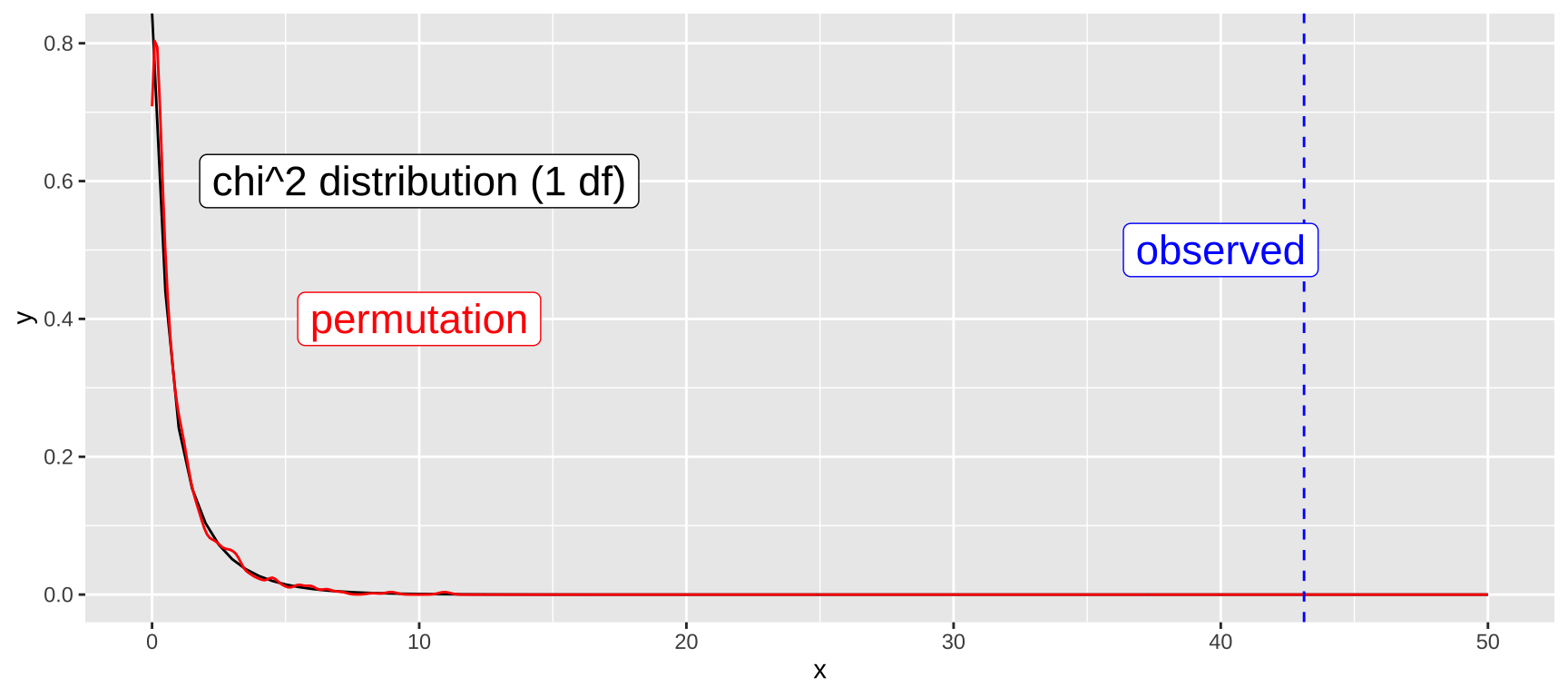

The plot above suggests a very low p-value, consistent with the results from our permutation test. We can also calculate this directly in R using the \(\chi^2\) test on the contingency table:

penguins_binary %>%
    select(Adelie, Biscoe) %>% # Turn our data into a contingency table
  table() %>% 
  chisq.test(correct = FALSE)

    Pearson's Chi-squared test

data:  .
X-squared = 43.118, df = 1, p-value = 5.154e-11

Quiz

Figure 9: The accompanying quiz link