R Recipes: Doing math in R, Using R functions, following Rs naming rules, and Importing data from a .csv.There are numerous embedded videos and associated quizzes which accompany this text. Make sure to watch them!
Motivating scenario: Motivating scenario: You have heard about R and RStudio, and maybe used them, but want a foundation so you can know whats going on as you do more and more with it.
Learning goals: By the end of this chapter you should be able to
- Explain why we are using R and RStudio.
- Describe the five tips for writing code like a pro.
- Install R and RStudio (or have access to them on RStudio cloud).
- Install the tidyverse package.
- Open and save an R script.
- Explain vectors, classes of variables, doing math, and asking logical questions in R.
Coding for biostats
Figure 1: Watch this video about why and how to R (6 min and 10 sec), from STAT 545 – a grad level data science class at the University of British Columbia. We will borrow from this course occasionally.
Writing, executing, and saving all steps of our data analysis allows us to share our scientific results. This makes our work reproducible and alllows people to borrow from, build off of, and evaluate what we have done. Be sure to watch the video above for high-level tips about how and why to use computer programs for reproducible science.
What is R and why / how do we use it?
R is a computer program, which is the go to language for most statisticians and data scientists (although some prefer python or julia). R makes it possible to conduct complex statistical analyses, make nice figures, and write this book, all in one environment.
As opposed to GUI’s, like Excel, or click-based stats programs, R is focused around writing and sharing scripts. This allows analyses to be shared and replicated, ensures that data manipulation occurs in a script, preserving the integrity of the original data, and allows for tremendous flexibility.
Why use R?
Figure 2: Watch this video about my intro to R videos, and about why and how we will use R. I will use these videos heavily for the first few weeks of course. You may have seen them elsewhere
- R is free.
- There are many “packages” in R for specialized analyses.
- R can make nice graphics.
- While learning R is not easy, inexperienced programmers can quite quickly do useful things. You will be able to make nice plots and summarize data by next week!
- Using R (or any scripting based analysis) allows us to save all the steps of our analysis, making our work easy to reproduce, describe, and build off of.
Observations and suggestions for learning R / computer stuff
Figure 3: Watch this video about keys to success in learing R
Teaching this class for years, I’ve learned a few things about learning R that you should know.
Observations
- Some people pick R up fast, other slowly.
- The speed at which students get familiar with R is unrelated to intelligence.
- Everyone who keeps trying gets there eventually.
- Despair and feeling low/dumb are the things that get people jammed up.
Suggestions
- Don’t worry. Keep trying. But TAKE BREAKS.
- Step away from the computer as much as possible, code & make plans on scratch paper.
- Be patient & understanding with yourself and your friends.
- Be creative.
- Ask for help.
- When something works (or it doesn’t) take time to figure out how / why.
- Fight the urge to compare yourself (negatively or positively) to others.
Today at the RStudio conference, Hadley Whickham, conrasted the “automatic negative thoughts” we feel some time in coding to the “balanced alternative” that we want to get to.
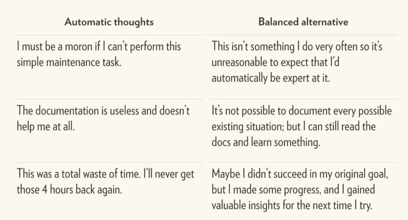
Figure 4: Complete this quiz about keys to success in learing R
What is RStudio?
More precisely, R is a programming language that runs computations, while RStudio is an integrated development environment (IDE) that provides an interface by adding many convenient features and tools. So just as the way of having access to a speedometer, rearview mirrors, and a navigation system makes driving much easier, using RStudio’s interface makes using R much easier as well.
Figure 5: Watch this video about accessing R and RStudio
You will see that there are many ways to do things in R. Over years of teaching this course I have switched to teaching predominantly using [tidyverse] tools.
One major reason for this is that the focus on a shared and coherent philosophy, grammar and data structure makes the tidyverse easier to teach and learn than base R. However, there are still challenges to learning and teaching the tidyverse, the two major challenges are
- It takes time to learn and appreciate the shared philosophy and data structure.
- Many people first learned R using base R, so it can be frustrating to start to learn again.
Installing R (or not)
We use R version 4.4.0 or above.
You can either download and install R, and RStudio, or you can do all the coursework with RStudio Cloud without installing anything on your computer (see Getting on RStudio Cloud for more info). Which option is right for you? It depends (see below). I suggest doing both and seeing which you prefer.
Getting on RStudio Cloud
Using RStudio Cloud allows you to use R and RStudio without installing anything on your computer. Additionally, if you log into our course project on RStudio Cloud you will not need to install any packages or load any files except those you want for fun or for your independent project at the end of term. Access it here.
Advantages to RStudio Cloud
From my experiencing teaching this course, about 5% of students have computers or computer systems where installing R is challenging, now you don’t have to.
Some students have older computers with limited computation. For them, a few class exercises (involving large-scale permutation or simulation) go super slow, and they can get justifiably frustrated.
Some computer setups make installing tidyverse or other specific R packages somewhat painful. RStudio Cloud removes this pain.
Using the course project guarantees that you’ll get the same environment as the prof and TA, making it easier for them to help you.
Disadvantages to RStudio Cloud
- The biggest disadvantage of RStudio cloud is that we might use R more than the free version allows (25 hours per month) and I would rather you not have to pay. That said, a student version is $5 a month (for 75 hours + an additional $0.10/hour) so it’s not so bad.
- Sometimes the system can get overwhelmed. This is pretty rare, but once a student was trying to use RStudioCloud during the international RStudio convention. The RStudio Cloud could not handle all the traffic and went down that day.
- You need an internet connection to use R. This can be a bummer if you don’t always have a reliable one.
- Some people (🖐) like having everything on their computer and struggle thinking about / working with folders on a cloud.
- Using the course project on RStudio Cloud might prevent you from learning how to load data, download packages etc.
Installing RStudio
First download/update R from here, be sure to download the version compatible with your computer, and pick any CRAN mirror you like (I usually do Iowa). If you installed R a while ago, be sure you’re using R version 4.4.0 or above.
Then download/update RStudio from here. Be sure to select the free version (RStudio Desktop, Open Source License), and as above, be sure to download the version compatible with your computer. If you installed RStudio a while ago, be sure you’re using the most recent RStudio Version: (2024.04.2+764).
Advantages to downloading and installing RStudio
- You can do a bunch without stable internet.
- You are not reliant on a cloud service which could go down.
- Everything is on your computer.
- You learn the joys (and frustrations, and how to overcome them) of dealing with packages, loading data etc… .
Disadvantages to downloading and installing RStudio
Figure 6: Take this quiz about accessing R and RStudio
The RStudio IDE
A tour of the Rstudio environment
Figure 7: My RStudio Overview link
Figure 8: My RStudio Quiz link
Intro to R
Using R as a calculator and for logical questions
R Recipe about Doing math in R
We can use R for simple math. For example:
# To add one and one
1 + 1 # will return
[1] 2# To square three
3^2 # will return[1] 9We can also use R for asking logical questions. For example:
# Is one greater than two?
1 > 2 # will return
[1] FALSE# Does four divided by four equal one?
4/4 == 1 # Note the two equals signs to ask the logical question[1] TRUE# Does four divided by four not equal one?
4/4 != 1 # Note an exclamation point then an equals sign means not equal.[1] FALSE# Is four divided by four greater than or equal to one?
4/4 >= 1 # Note greater than sign, then an equals sign means greater than or equal to[1] TRUE# in my r code before some words. The # tells R that we are not using R code here but rather we are providing a comment to make our code easier for people to understand. Commenting your code is great.
Vectors in R
Most of what we do in R starts with a vectors – a combination of simple entities. We already came across a few simple vectors of length one – for example, the number, 1 and the logical statement, TRUE, above.
Vectors are often longer than length one, for example, we can make a vector with the numbers one, five, and two with the c()oncatenate function as follows:
c(1, 5, 2) # which returns[1] 1 5 2Assigning variables in R
R Recipe about following Rs naming rules
Figure 9: Assignment and good names for things video link
Figure 10: Assignment and good names for things quiz link
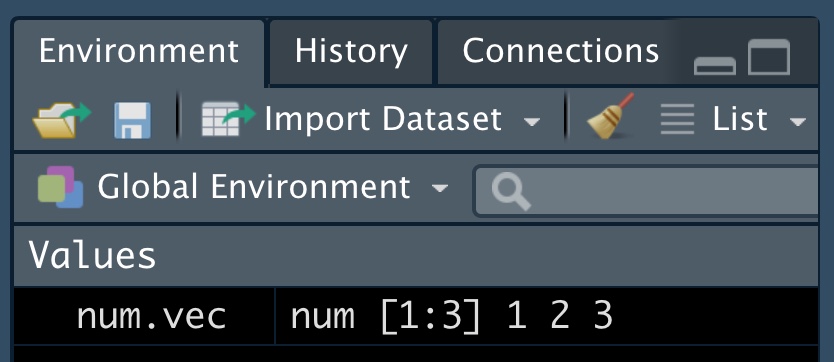
Use the assignment operator <- to assign values to a variable. For example
num_vec <- c(4, 9, 16)With these variables assigned, we can do simple math, ask logical questions , use them as arguments for functions. For example sqrt(x = num_vec) returns 2, 3, 4. All variables assigned should be in your environment window (see below).
sqrt(x = num_vec) is the same as sqrt(num_vec) and with just one argument (x) for the function, this is totally unnecessary. When there are more arguments it is good practice to include the argument name and the equals sign, as this makes code easier to read, and more likely to work (otherwise R assumes we put things in a specific order).
Using functions in R
R Recipe on Using R functions.
Figure 11: Using Rs functions link
Only so much can be done with simple math. We can do more complex analyses in R with functions. Functions take in arguments and return some output. Here are some simple examples:
- To get the mean of a vector, use the
mean()function.
- To get the length of a vector, use the
length()function.
- Use the
help()function to learn more about a given function. For examplehelp(length)will return this (Fig: 12).
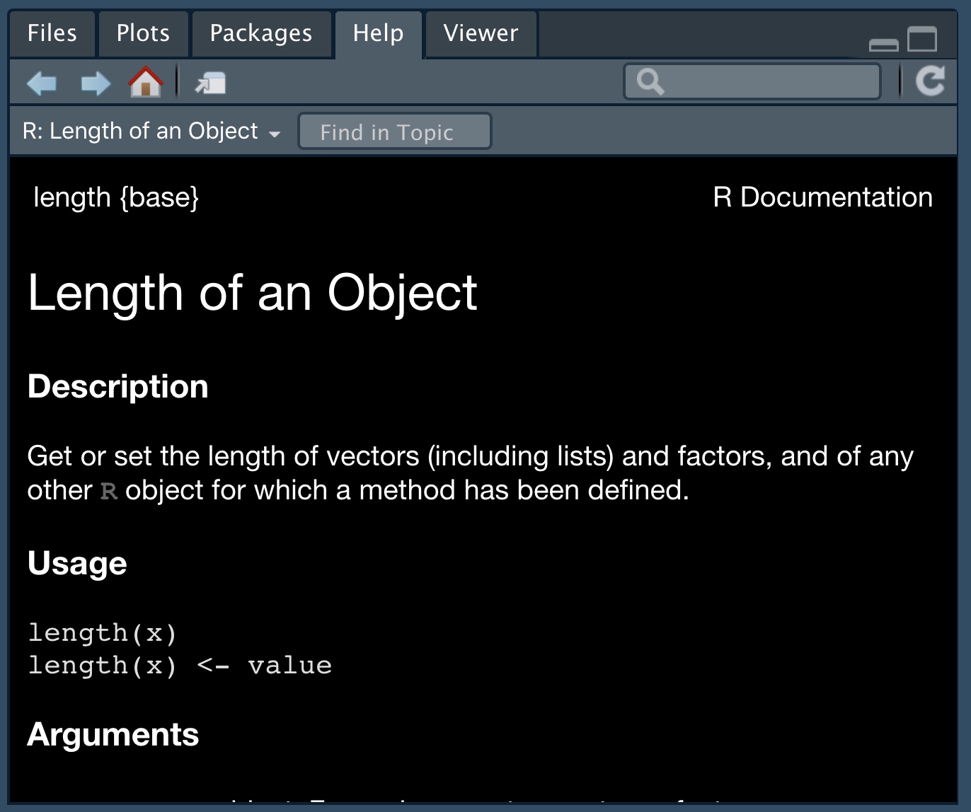
Figure 12: An example of R help
Throughout the text, I include a hyperlink to the help for every function I introduce. There is no need to look into all of these, but it is a good practice to look at the when you are confused. Unfortunately it takes a bit of practice / knowledge to make sense of R’s help. So, check out this reference to figure out how to get the most from R’s help.
The tab button is very useful when we deal with functions. Hitting tab as you begin to type a function’s name will give suggested functions, with a brief description, while hitting tab inside the parentheses of a function will show the arguments the function takes.
Figure 13: A quiz about using functions in R
Packages
Figure 14: Using, installing, and loading Rs functions link
While R has many useful built-in “base” functions, and advanced R users can write their own specialized functions, many people have developed suites of useful additional functions to extend R to do a bunch of stuff.
- The first time we want to used a package, we install is with with the
install.packages()function. So, for example, to install the readr and readxl packages (which are useful for reading in data), type”
install.packages("readr")           # quotes required
install.packages("readxl") # quotes required- After our initial install, we need need install the package again (although we may want to update it), but we do need to load each package we use each time we restart
R. Use thelibrary()function to do so. So, for example, to install the readr and readxl packages, type:
Figure 15: A quiz about using, installing, and loading R packages
Loading data in R
R Recipe about Importing data from a .csv.
Sadly, while loading data into R is the first step for any analysis it requires much R knowledge and numerous R skills. This is why we have waited until introducing this. Yet I think we’re ready. One challenge of loading data is that you have to tell R where your data is. So the first way I’ll teach you to do this is by getting data off the internet. In this case, we just give R the link to the data. Next I’ll show you how to read get data from your computer. In both cases we’ll use the read_csv() function in the readr package to load data. This assumes you have a .csv file. You can similarly use the read_excel() function if you have an excel file (check out this recipe if you want to know more).
To load data in this way
- Make sure the
readrpackage is installed and loaded.
- Type
read_csv(FILE_LOCATION), where theFILE_LOCATIONpointsRto the file.
- Use the assignment operator to make sure
Rkeeps the data in its memory
# NOTE: Both ALL_CAPS things below should be replaced by appropriate names
NAME_OF_VARIABLE_FOR_DATA <- read_csv(FILE_LOCATION)
Loading data from the internet.
Figure 16: Loading data into R from the internet link. We use the compensation data, available here https://raw.githubusercontent.com/ybrandvain/datasets/master/compensation.csv
It’s quite easy to tell R where data is on the internet, just show it the link! Note the link can be a character variable. For example:
link_to_data <- "https://figshare.com/articles/dataset/long_and_complex_link_this_one_is_fake_and_wont_work.csv"
fake_data    <- read_csv(link_to_data)
Figure 17: A quiz about loading data into R form the internet
Loading data from your computer.
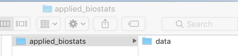
We aren’t always lucky enough to have data on the internet. In fact when we are conducting our own science, we save data onto our computer. This makes finding the data and directing R to it somewhat difficult. Although there are may ways to do this, I find that making a project and having simple and consistent folder organization make this easiest. In general, I make a new Rproject, for each new research project. In this course, you might want to make one R project for standard classwork and standard homework, and distinct Rprojects for your more involved evaluations. But see what works best for you. To get started
- Make a folder for this course (whatever you want to call it) and include a sub-folder called data
- Open
Rright now and make a project in the existing folder that contains the subfolder, data (it will get the same name),
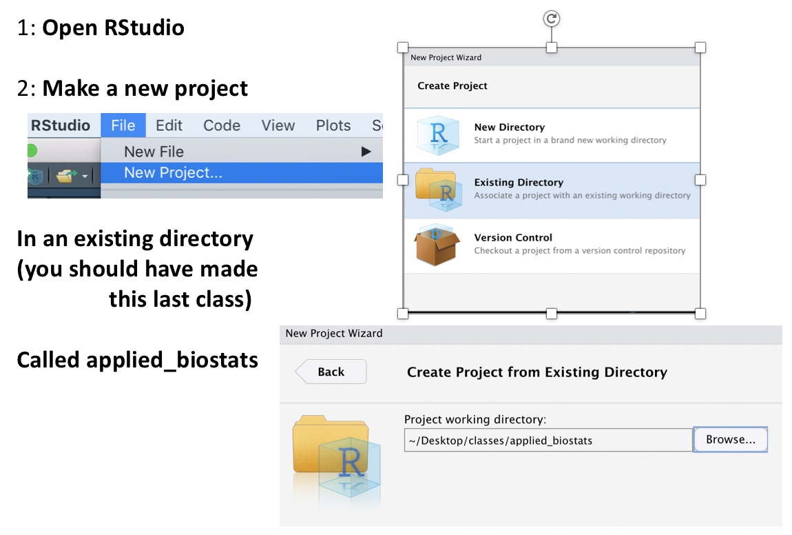
This makes loading data way easier (see the video below)
Figure 18: Making a project and loading data from your computer into R link
Looking into your data
Figure 19: Looking into R data link. We use the compensation data as an example.
The first thing to do once we’ve loaded our data is to examine it. Often when R does not work as we expected because the data aren’t as we expected. When looking at a data, recall that all columns in a tibble are vectors, and all entries in a vector must be of the same class. The three most relevant classes are:
numeric– Contains numbers which can take any value. For examplec(1, 2, 3)returns1, 2, 3.
logical– Contains logical statements. For example,c(TRUE, FALSE, FALSE)returnsTRUE, FALSE, FALSE.
character– Contains letters, words, and/or phrases. For examplec("The dog", "jumped", "over", "the moon")returnsThe dog, jumped, over, the moon.
You may also come across two other classes of vectors:
factor– This is a lot like a character, with the caveat that they are coded by numbers in R’s brain (see below). This can sometimes make things tough, so be careful, and consider when things are not working right that maybe you have factor when you thought you had a character.
integer– A number that must take an integer value. For exampleas.integer(c(1, 2.1, 3))returns1, 2, 3.
We will use the glimpse() function in the dplyr package to look into our data. So make sure you have the dplyr package installed and loaded. In later chapters we’ll learn how use the mutate() function in dplyr to change between data types in the case in which R has the wrong idea.
(#fig:looking_at_data-quiz)A quiz about looking into our data in R
Making exploratory plots
Figure 20: Simple exploratory plots with the GWalkR GUI. video link. We use the compensation data for this example.
Another very important way to look at your data is to plot it! This is always the first step in a data analysis in that it helps us understand our data and scan for outliers. Later we will learn how to use the ggplot2 package in R to make high-quality and reproducible plots. But that is not our goal today. Today we hope to quickly explore our data with minimal coding skill. To do so we will use the gwalkr() function in the GWalkR package to bring up a simple GUI to explore our data. Remember to install the GWalkR package the first time you use it, and load the library every time you restart R.

R scripts
Figure 21: Document R work by saving R scripts link
A great thing about R is that you can remember and share exactly what you have done by saving your work as a script. In doing so it’s best practice to type your name, date and the goal of the analysis at the top (with a # to tell R this isn’t code), plus a description of your goals. Regular comments throughout, help make your code more usable.
To make a new R Script, click on File, then New File, and then R Script.
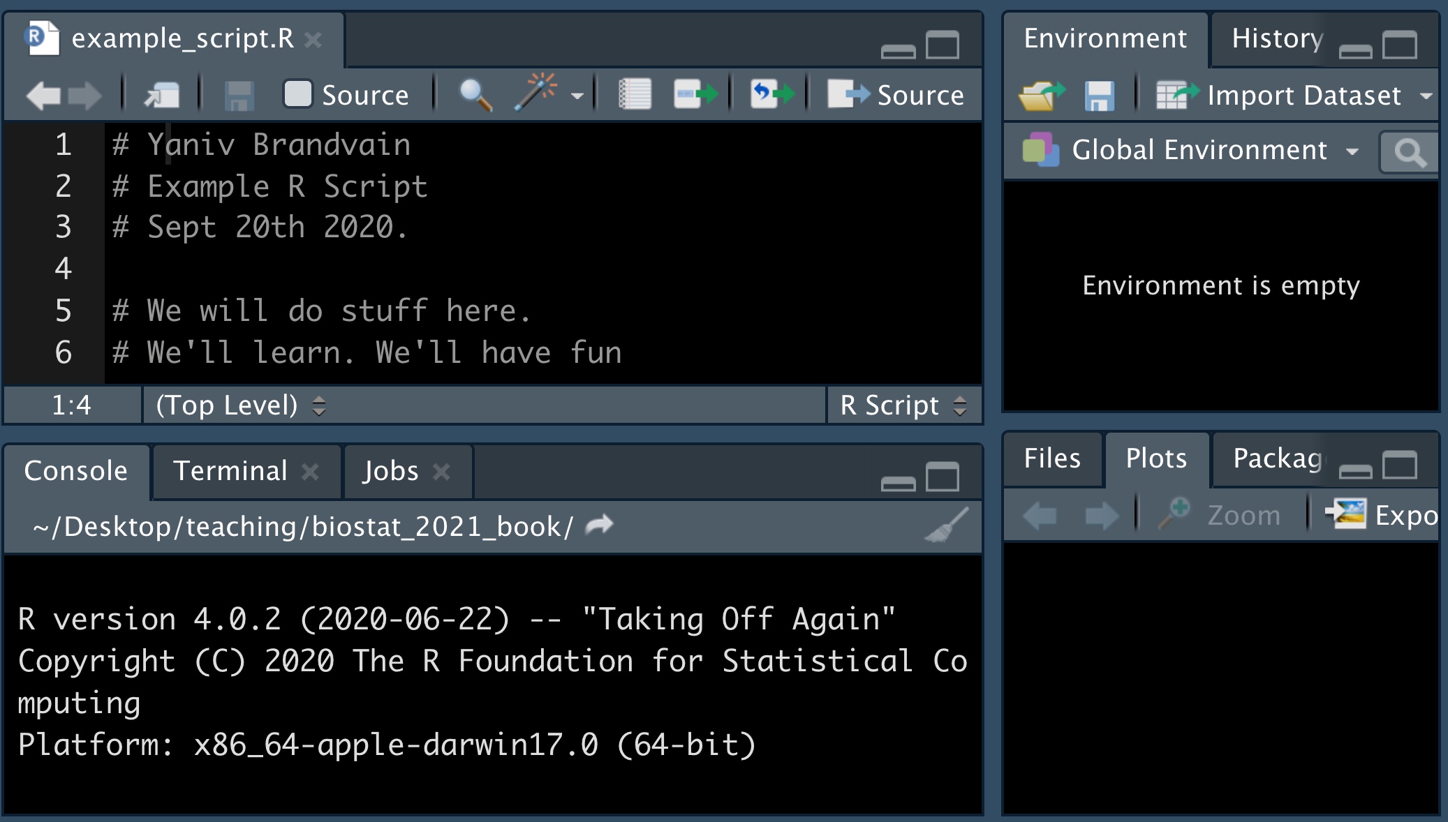
Figure 22: A quiz about composing good Rscripts