There are a few fiddly things we haven’t covered yet, that you might need to know. Here I let you know them. Throughout I use the iris dataset as an example with:

x = Sepal.Width.
y = Petal.Width.
Species as a categorical predictor

Plotting with Parallel Slopes

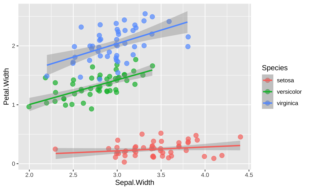
It’s good practice for your figures to visually reflect the statistical model you’ve fitted. Unfortunately, this can sometimes be challenging in ggplot2. By default, ggplot2 will fit a separate slope for each category in a grouping variable, as shown below:

iris %>%
  ggplot(aes(x = Sepal.Width, y = Petal.Width, color = Species)) +
  geom_jitter(height = 0.1, width = 0.02, alpha = 0.7, size = 3) +
  geom_smooth(method = "lm")

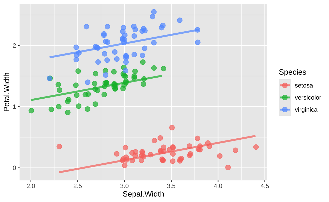
To enforce parallel slopes, we can use predictions from a linear model (obtained using the augment function from the broom package) and plot these predictions with geom_line().

lm(Petal.Width ~ Sepal.Width + Species, data = iris) %>%
  augment() %>%
  ggplot(aes(x = Sepal.Width, y = Petal.Width, color = Species)) +
  geom_jitter(height = 0.1, width = 0.02, alpha = 0.7, size = 3) +
  geom_line(aes(y = .fitted), size = 1.3, alpha = 0.7)

This approach ensures that the plot reflects a model with parallel slopes across species by using the fitted values from a model without interaction terms, resulting in lines with shared slopes across groups.

Post hoc tests for interaction terms

Say that I wanted to include an interaction term in my model. We can see a significant interaction below.

model_with_interaction <- lm(Petal.Width ~ Sepal.Width * Species, data = iris)
Anova(model_with_interaction, type = "II")

Anova Table (Type II tests)

Response: Petal.Width
                    Sum Sq  Df   F value    Pr(>F)    
Sepal.Width          1.363   1   46.5846 2.264e-10 ***
Species             70.172   2 1199.0878 < 2.2e-16 ***
Sepal.Width:Species  0.580   2    9.9109 9.276e-05 ***
Residuals            4.214 144                        
---
Signif. codes:  0 '***' 0.001 '**' 0.01 '*' 0.05 '.' 0.1 ' ' 1

summary(model_with_interaction)                                                                                                                                                                               %>% coef() %>% data.frame()%>% rownames_to_column(var = "Species")%>% mutate_at(-1,round, digits = 5)%>% rename("P_value"="Pr...t..")

                        Species Estimate Std..Error t.value P_value
1                   (Intercept)  0.02418    0.22231 0.10876 0.91354
2                   Sepal.Width  0.06471    0.06447 1.00376 0.31718
3             Speciesversicolor  0.14273    0.31071 0.45936 0.64667
4              Speciesvirginica  0.63988    0.31747 2.01554 0.04571
5 Sepal.Width:Speciesversicolor  0.35374    0.10110 3.49905 0.00062
6  Sepal.Width:Speciesvirginica  0.39324    0.09949 3.95272 0.00012

Remember that these p-values are not exactly what we want:

The p-value for the intercept tests the nonsensical null hypothesis that the Petal Width of setosa plants with a Sepal Width of zero is equal to zero.
The p-value for Sepal Width, while testing a somewhat reasonable null (that the slope is zero), is challenging to interpret. It differs from the results we obtain using Type II sums of squares with our full model.
The p-values for Speciesversicolor and Speciesvirginica test the null hypothesis that their intercepts are identical to that of setosa. However, they are somewhat miscalibrated and do not allow us to compare versicolor and virginica directly.
The p-values for Sepal.Width:Speciesversicolor and Sepal.Width:Speciesvirginica test the null hypothesis that their slopes are identical to that of setosa. Like the intercept comparisons, these are also somewhat miscalibrated and do not allow us to compare versicolor and virginica slopes directly.

Post hoc tests

To address these limitations, we conduct post hoc tests! We have seen this approach with a categorical variable before.

emmeans(model_with_interaction, ~ Species)

 Species    emmean    SE  df lower.CL upper.CL
 setosa      0.222 0.034 144    0.155    0.289
 versicolor  1.446 0.033 144    1.381    1.511
 virginica   2.064 0.025 144    2.015    2.114

Confidence level used: 0.95

# Print the results
emmeans(model_with_interaction, ~ Species) %>%
  pairs(., adjust = "tukey")

 contrast               estimate     SE  df t.ratio p.value
 setosa - versicolor      -1.224 0.0474 144 -25.854  <.0001
 setosa - virginica       -1.842 0.0422 144 -43.647  <.0001
 versicolor - virginica   -0.618 0.0414 144 -14.939  <.0001

P value adjustment: tukey method for comparing a family of 3 estimates

Now we can do this for our interactions too

emmeans(model_with_interaction, ~ Species * Sepal.Width)

 Species    Sepal.Width emmean    SE  df lower.CL upper.CL
 setosa            3.06  0.222 0.034 144    0.155    0.289
 versicolor        3.06  1.446 0.033 144    1.381    1.511
 virginica         3.06  2.064 0.025 144    2.015    2.114

Confidence level used: 0.95

# Print the interaction estimates
emmeans(model_with_interaction, ~ Species * Sepal.Width,at = list(Sepal.Width = 0)) %>%
  contrast(method = "pairwise", adjust = "tukey")                                                                                  %>% data.frame()%>%select(-SE,- df, -t.ratio)%>% mutate_at(-1,round, digits = 3)

                                          contrast estimate p.value
1    setosa Sepal.Width0 - versicolor Sepal.Width0   -0.143   0.890
2     setosa Sepal.Width0 - virginica Sepal.Width0   -0.640   0.112
3 versicolor Sepal.Width0 - virginica Sepal.Width0   -0.497   0.256

Effect sizes in ANOVAs and ANCOVAs etc

We know that statistical significance is not a reliable measure of effect size.

For simple models (e.g., a t-test), we can calculate summaries like Cohen’s D (the difference between groups divided by the standard deviation) as a measure of effect size.
For a simple regression, the correlation coefficient, \(r\), is a useful measure of the effect of a predictor variable.
In multiple regression, we can find the standardized regression coefficients (similar to the slopes) by \(Z\)-transforming our variables. Note: The example below is illustrative, but multicollinearity can lead to unreliable standardized coefficients, so don’t make much of the fact that these are greater than one and less than negative one

# Example with Z-transformed variables in a multiple regression
iris %>% 
  select(1:3) %>%
  mutate_all(scale,center = TRUE,scale = TRUE) %>% # z transform
  lm(Sepal.Width ~ Sepal.Length + Petal.Length, data = .) %>%
  coef()

  (Intercept)  Sepal.Length  Petal.Length 
 8.545613e-16  1.066151e+00 -1.357861e+00

Effect Size in an ANCOVA

When we have a mix of categorical and continuous predictors in our model, describing effect size requires careful consideration.

Partial \(R^2\)

Partial \(R^2\) is a measure of effect size in a general linear model. It describes the proportion of variance in \(y\) that is uniquely explained by a specific explanatory variable. Like the standard \(R^2\), partial \(R^2\) is calculated as the sums of squares attributable to the “model” divided by the sums of squares “total.” However, for partial sums of squares, the “model” consists only of the variable of interest (using Type III sums of squares), and the “partial sums of squares total” is defined as the residual sums of squares plus the sums of squares for the focal explanatory variable:

We can obtain this directly from the Type III ANOVA output in R:

ss_error <- Anova(model_with_interaction, type = "III")%>% 
  tidy() %>% 
  filter(term =="Residuals")%>%
  pull(sumsq)


Anova(model_with_interaction, type = "III")%>% 
  tidy() %>%
  mutate(partial_r2 = sumsq/ (sumsq+ss_error))%>%
  filter(!term %in% c("(Intercept)", "Residuals"))                                                                                                             %>% 
  mutate_at(-1, round , digits = 4) %>% gt()

term	sumsq	df	statistic	p.value	partial_r2
Sepal.Width	0.0295	1	1.0075	0.3172	0.0069
Species	0.1307	2	2.2335	0.1109	0.0301
Sepal.Width:Species	0.5800	2	9.9109	0.0001	0.1210

Standardized regression coefficients:

We can obtain “standardized regression coefficients” by z-transforming all continuous predictors and the continuous response, as shown below. However, interpreting these coefficients can be challenging in the presence of a categorical predictor, as the effects of the categorical predictor are expressed in units of the standard deviation of the response.

iris %>%
  mutate(across(where(is.numeric), ~ (.- mean(.)) / sd(.))) %>%
  lm(Petal.Width ~ Sepal.Width * Species, data = .) %>%
  summary() %>%
  tidy()                                                                                                                                                 %>% select(term, estimate, std.error)%>% mutate(across(where(is.numeric), round, digits = 3))  %>% gt()

term	estimate	std.error
(Intercept)	-1.282	0.045
Sepal.Width	0.037	0.037
Speciesversicolor	1.606	0.062
Speciesvirginica	2.417	0.055
Sepal.Width:Speciesversicolor	0.202	0.058
Sepal.Width:Speciesvirginica	0.225	0.057

Homework

For your homework write a two to three paragraph summary of your analysis and results so far (in th linear model framework). Include summary stats, 1-2 plots, and a description of your motivation, methods, results, interpretation and conclusion. Finally, add any questions you want help with or things you hope to do that cannot yet accomplish.

When you are done share the here.

Note you will be exchanging these with other class members friday.

Chapter 31: Bits & Bobs