Motivating scenario: We start at the beginning of a study – how do we set up a good way to keep track of data that will allow us to focus on understanding and analyzing our data, not reorganizing and rearranging it?
Learning goals: By the end of this chapter you should be able to
- Make a data sheet.
- Label samples.
- Describe best principles for collecting, storing, and maintaining data.
- Explain why these are good ideas.
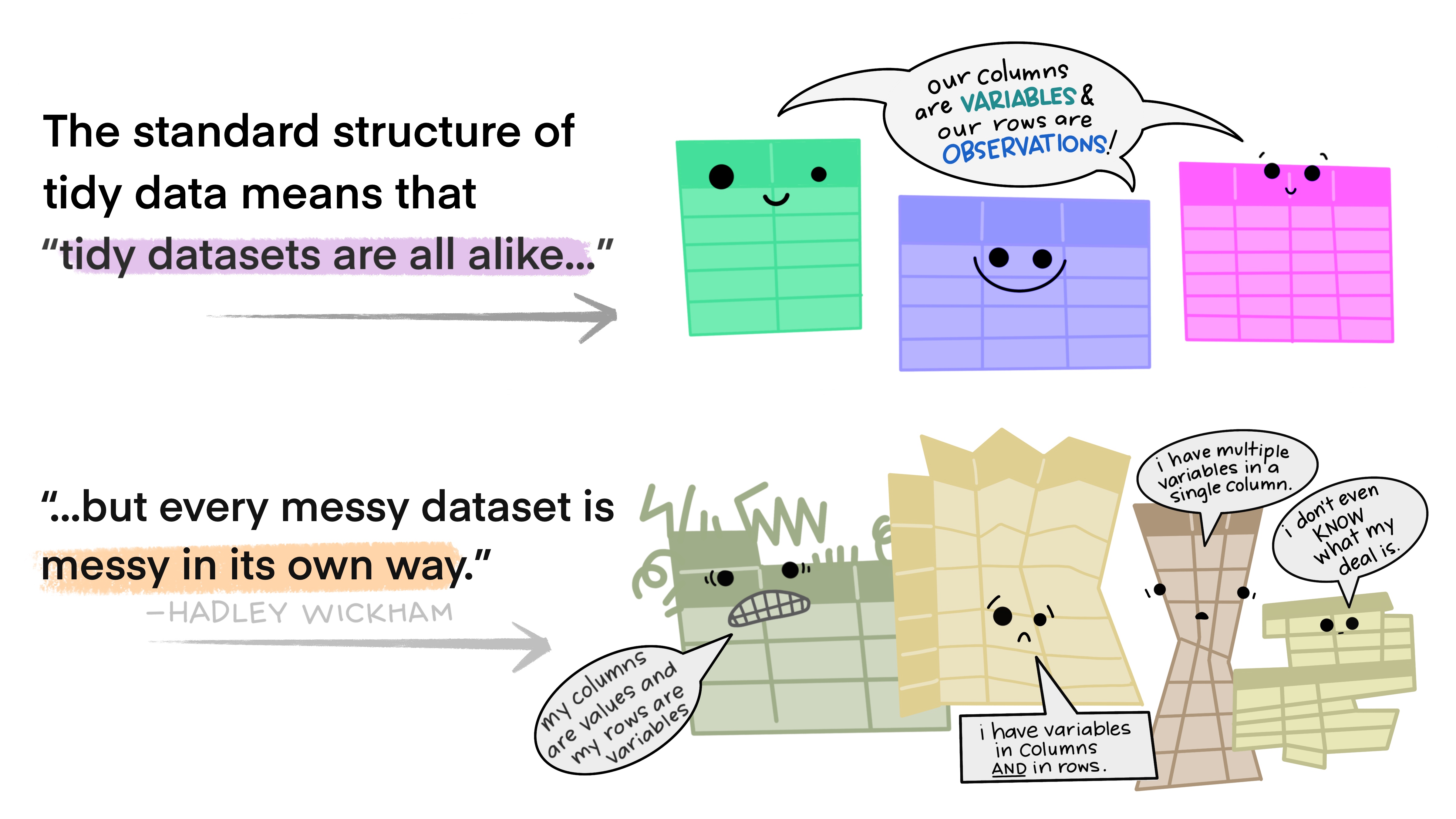
- Differentiate between tidy and messy data.
- Load data into R using a project
(1) Data Organization in Spreadsheets (Broman and Woo 2018).
(2) Tidy Data (Wickham 2014).
(3) Ten Simple Rules for Reproducible Computational Research (Sandve 2013).
We care about the data, the data are our guide through this world. It is therefore very important to ensure the integrity of our data. Kate Laskowski learned this all too well, when her collaborator messed with her data set. In the required video below, she outlines the best practices to ensure the integrity of your data, both against unscrupulous collaborators, or, more likely, minor mistakes introduced in the process of data collection and analysis.
Figure 1: Kate Laskowski on data integrity (6 min and 06 seconds).
Organizing folders.
Keeping data organized will make your life better. Give each project its own folder, with sub-folders for data, figures, code, and writing. This makes analyses easy to share and reproduce. Before taking any data, get your folders in order!
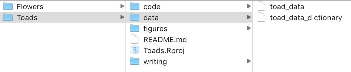
Figure 2: Example folder structure
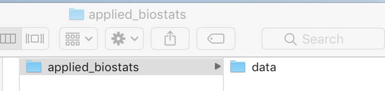
I highly recommend treating this course as a project, so make a folder on your computer called applied_biostats and a folder in there called data. If you do this, your life will be better. You might even want to do one better and tret each class session as a project.
Collecting data.
On two occasions I have been asked, “Pray, Mr. Babbage, if you put into the machine wrong figures, will the right answers come out?” … I am not able rightly to apprehend the kind of confusion of ideas that could provoke such a question.
Page 64 of “Passages from the Life of a Philosopher” by Charles Babbage (1864)
Sometimes, data come from running a sample through a machine, resulting in a computer readout of our data (e.g., genotypes, gene expression, mass spectrometer, spectrophotometer, etc.). Other times, we collect data through counting, observing, and similar methods, and we enter our data by hand. Either way, there is likely some key data or metadata for which we are responsible (e.g., information about our sample). In this chapter, we focus on how we collect and store our data, assuming that our study and sampling scheme have already been designed. Issues in study design and sampling will be discussed in later chapters.
Making rules for data collection
Before we collect data, we need to decide what data to collect. Even in a well-designed study where we want to observe flower color at a field site, we must consider, “What are my options?” (i.e., “How do I code my data?”). Should the options be “white” and “pink,” or should we distinguish between darker and lighter shades? If we’re measuring tree diameter, at what height on the tree should we measure the diameter? When measuring something quantitative, what units are we reporting? Some of these questions have answers that are more correct, while for others, it’s crucial to agree on a consistent approach and ensure each team member uses the same method. Similarly, it’s important to have consistent and unique names – for example, my collaborators and I study Clarkia plants at numerous sites – include Squirrel Mountain and SawMill – which one should we call SM (there is a similar issue in state abbreviation – we live in MiNnesota (MN), not MInnesota, to differentiate our state from MIchigain (MI)). These questions highlight the need for thoughtful data planning, ensuring that every variable is measured consistently.
Once you have figured out what you want to measure, how you will measure and report it, and other useful info (e.g., date, time, collector), you are ready to make a data sheet for field collection, a database for analysis, and a README or data dictionary.
Making a spreadsheet for data entry
After deciding on consistent rules for data collection, we need a standardized format to enter the data. This is especially important when numerous people and/or teams are collecting data at different sites or years. Spreadsheets for data entry should be structured similarly to field sheets (described below) so that it is easy to enter data without needing too much thought.
Some information (e.g., year, person, field site) might be the same for an entire field sheet, so it can either be written once at the top or explicitly added to each observation in the spreadsheet (copy-pasting can help here).
Data validation
When making a spreadsheet, think about future-you (or your collaborator) who will analyze the data. Typos and inconsistencies in values (e.g., “Male,” “male,” and “M” for “male”) aren’t the end of the world but create unnecessary headaches. Accidentally inputting the wrong measure (e.g., putting height where weight should be, or reporting values in kg rather than lb) can be a much bigger hassle. Both Excel and Google Sheets (and likely most spreadsheet programs) have a simple solution: use the “Data validation” feature in the “Data” drop-down menu to limit the potential categorical values or set a range for continuous values that users can enter into your spreadsheet. This helps ensure the data are correct.
Making a README and/or “data dictionary”
A data dictionary is a separate file (or sheet within a file, if you prefer) that explains all the variables in your dataset. It should include the exact variable names from the data file, a version of the variable name that you might use in visualizations, and a longer explanation of what each variable means. Additionally, it is important to list the measurement units and the expected minimum and maximum values for each variable, so anyone using the data knows what to expect.
Alongside your data dictionary, you should also create a README file that provides an overview of the project and dataset, explaining the purpose of the study and how the data were collected. The README should include a description of each row and column in the dataset. While there may be some overlap with the data dictionary, this is fine. The data dictionary can serve as a quick reference for plotting and performing quality control, whereas the README provides a higher-level summary, designed for those who may not have been directly involved in the project but are seriously interested in the data.
![Example data dictionary from [@broman2018].](http://www.tandfonline.com/cms/asset/a0ee9bd4-ec62-4aa0-85cd-ef3514ba63bd/utas_a_1375989_f0009_b.jpg)
Figure 3: Example data dictionary from (Broman and Woo 2018).
Making Data (field) sheets
When collecting data or samples, you need a well-designed data (field) sheet. The field sheet should closely resemble your spreadsheet but with a few extra considerations for readability and usability. Ask yourself: How easy is this to read? How easy is it to fill out? Each column and row should be clearly defined so it’s obvious what goes where. Consider the physical layout too—does the sheet fit on one piece of paper? Should it be printed in landscape or portrait? Print a draft to see if there’s enough space for writing. A “notes” column can be useful but should remain empty for most entries, used only for unusual or exceptional cases that might need attention during analysis.
It’s also smart to include metadata at the top—things like the date, location, and who collected the data. Whether this metadata gets its own column or is written at the top depends on practical needs—if one person is responsible for an entire sheet, maybe it belongs at the top, not repeated for every sample (unlike what is done in Figur Figure @ref(fig: datasheet)).
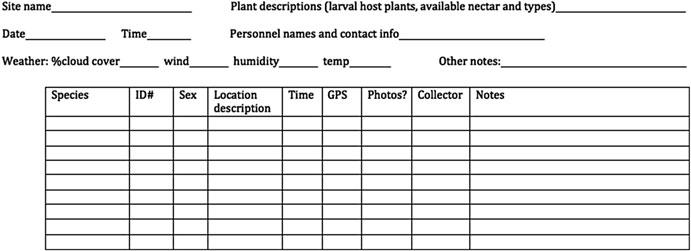
Figure 4: An example data sheet for collecting plant samples.
Backing up data sheets
After collecting data, you should first take a picture of and/or scan your data sheet. Store this digital copy in a folder with your data sheet to ensure it won’t be misplaced. Then store the physical data sheet in a reliable place (e.g., a physical folder, not just a random spot), so you have a backup even if the digital version is deleted.
Entering data sheets into a computer
Enter the data as soon as possible. Once the data is entered, lock it (either the entire file if you’re done with data entry or the data entered so far if you’re not). Then keep one copy on your physical computer and another on the cloud that’s shared with your collaborators. The two files should be identical. If multiple teams collect data at different times and sites, decide whether the data are best kept in one sheet or several sheets that can be combined later. If you choose the second option, ensure the spreadsheets follow the same rules and formats, and include columns that differentiate the spreadsheets (e.g., Year, University).
Additional guidence for spreadshets
Be consistent and deliberate
You should refer to a thing in the same thoughtful way throughout a column. Take, for example, gender as a nominal variable. Data validation approaches (above, can help).
A bad organization would be: male, female, Male, M, Non-binary, Female.
A good organization would be: male, female, male, male, non-binary, female.
A just as good organization would be: Male, Female, Male, Male, Non-binary, Female.
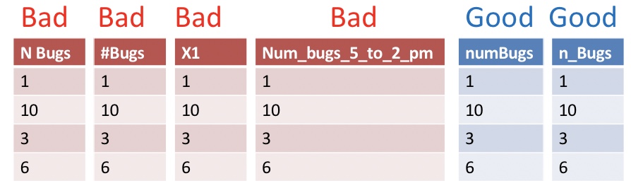
Use good names for things
Names should be concise and descriptive. They need not tell the entire story. For example, units are better kept in a data dictionary (below) than column name. This makes downstream analyses easier.
Backup your data, do not touch the original data file and do not perform calculations on it.
We discussed the importance o saving your data on both your computer and a locked, un-editable location on the cloud (e.g. google docs, dropbox, etc.). When you want to do something to your data do it in R, and keep the code that did it. This will ensure that you know every step of data manipulation, QC etc/
🤔 Why? 🤔 Your data set is valuable. You don’t want anything to happen to it. It also could allow you to ensure that your collaborators (and/or former house-mates) did not manipulate the data.
Data should be tidy (aka rectangular)
Ideally data are tidy this means
- Each variable must have its own column.
- Each observation must have its own row.
- Each value must have its own cell.
That said - you must balance two practicle considerations – “What is the best way to collect and enter data?” vs “What is the easiest way to analyze data?” So consider the future computational pain of tidying untidy data when ultimately deciding on the best way to format your spreadsheet (above).
Loading A Spreadsheet into R
Getting data into R is often the first challenge we run into in our first R analysis. I review how to do this below.
- Ideally, your data are stored as a
.csv, and if so you can read data in with theread_csv()function.Rcan deal with other formats as well. Notably, using the functionreadxl::read_excel()allows us to read data from Excel, and can take the Sheet of interest as an argument in this function.
- Ideally you have made an R project, for this work. As it makes loading data easier.
Here’s an example of how to read data into R. To start we open Toads.Rproj by either
- Opening RStudio by opening
Toads.Rprojor - Clicking
Fileand navigating toOpen projectonce RStudio is open.
Opening Toads.Rproj tells RStudio that this is our home base. The bit that says data/ points R to the correct folder in our base, while toad_data.csv refers to the file we’re reading into R. The assignment operator <- assigns this to toad_data. Using tab-completion in RStudio makes finding our way to the file less terrible. But you can also point and click your way to data (see below). If you do, be sure to copy and paste the code you see in the code preview into the script so you can recreate your analysis..
Dealing with (other people’s) data in spreadsheets
We are often given data collected by someone else (collaborators, open data sets etc). If we’re lucky they did a great job and we’re ready to go. More often, they did ok and we have a painful hour to a painful week ahead of us as we clean up their data. Rarely, their data collection practices are so poor that their data are not useful.
In this course we will cover some basic data wrangling tools to deal with ugly datasets, but that is not a course focus or course goal. So, our attention to this issue will be minimal. If you want more help here, I suggest part II of R for Data Science (Grolemund and Wickham 2018).
Tidying messy data
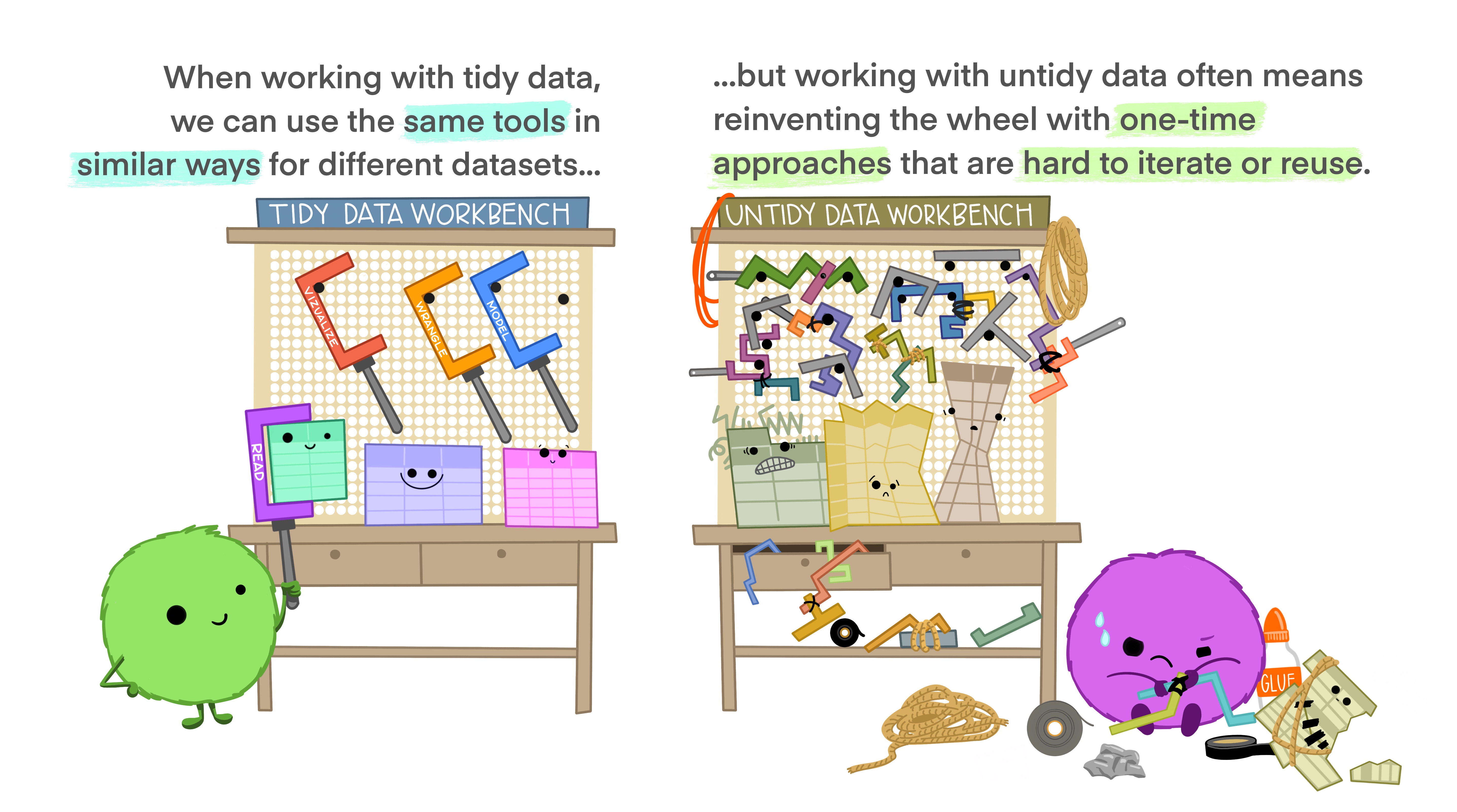
Figure 5: Tidy tools require tidy data
Above, we said it is best to keep data in a tidy format, and in previous chapters we noted that Tidyverse tools have a unified grammar and data structure. From the name, tidyverse, you could probably guess that tidyverse tools require tidy data – data in which every variable is a column and each observation is a row. What if the data you loaded are untidy? The pivot_longer function in the tidyr package (which loads automatically with tidyverse) can help! Take this example dataset, about grades in last year’s course.
# A tibble: 2 × 4
  last_name first_name exam_1 exam_2
  <chr>     <chr>       <dbl>  <dbl>
1 Horseman  BoJack       35     36.5
2 Carolyn   Princess     48.5   47.5
This is not tidy. If it were tidy each observation would be a score on an exam. So we need to move exam to another column. We can do this!!!
library(tidyr)
tidy_grades <-pivot_longer(data = grades, # Our data set
             cols = c(exam_1, exam_2),    # The data we want to combine
             names_to = "exam",           # The name of the new column in which we put old names.
             values_to = "score"          # The name of the new column in which we put the values.
             )

tidy_grades
# A tibble: 4 × 4
last_name first_name exam score
<chr> <chr> <chr> <dbl>
1 Horseman BoJack exam_1 35
2 Horseman BoJack exam_2 36.5
3 Carolyn Princess exam_1 48.5
4 Carolyn Princess exam_2 47.5This function name, pivot_longer, makes sense because another name for tidy data is long format. You can use the pivot_wider function to get data into a wide format.
Learn more about tidying messy data in Fig. 6:
Figure 6: Tidying data (first 5 min and 40 seconds are relevant).
Quiz
Figure 7: The accompanying getting data quiz link.