Learning goals: By the end of this chapter you should be able to
- Describe what a linear model is, and what makes a model linear.
- Connect the math of a linear model to a visual representation of the model.
- Use the
lm()function in R to run a linear model and thecoef()function to interpret its output to make predictions.
- Understand what a residual is
- Be able to calculate a residual.
- Visually identify residuals in a plot.
- Be able to calculate a residual.
- Recognize the limitations of predictions form a linear model.
- Get a sense for what makes a linear model “good” or “bad”.
Linear models describes the predicted value of a response variable as a function of one or more explanatory variables. The predicted value of the response variable of the \(i^{th}\) observation is \(\hat{Y_i}\), where the hat denotes that this is a prediction. This prediction, \(\hat{Y_i}\) is a function of values of the explanatory variables for observation \(i\) (Equation (1)). We have already spent some time in the last section with a very common linear model – a linear regression.
\[\begin{equation} \hat{Y_i} = f(\text{explanatory variables}_i) \tag{1} \end{equation}\]
A linear model predicts the response variable by adding up all components of the model. So, for example, \(\hat{Y_i}\) equals the parameter estimate for the “intercept”, \(a\) plus its value for the first explanatory variable, \(y_{1,i}\) times the effect of this variable, \(b_1\), plus its value for the second explanatory variable, \(y_{2,i}\) times the effect of this variable, \(b_2\) etc all the way through all predictors (Eq. (2)).
\[\begin{equation} \hat{Y_i} = a + b_1 y_{1,i} + b_2 y_{2,i} + \dots{} \tag{2} \end{equation}\]
Linear models can include e.g. squared, and geometric functions too, so long as we get out predictions by adding up all the components of the model. Similarly, explanatory variables can be combined – so we can include cases in which the effect of explanatory variable two depends on the value of explanatory variable one, by including an interaction in the linear model.
Optional: A view from linear algebra
If you have a background in linear algebra, it might help to see a linear model in matrix notation.
The first matrix in Eq (3) is known as the design matrix. Each row corresponds to an individual, and each column in the \(i^{th}\) row corresponds to this individual \(i\)’s value for the explanatory variable in this row. We take the dot product of this matrix and our estimated parameters to get the predictions for each individual. Equation (3) has \(n\) individuals and \(k\) explanatory variables. Note that every individual has a value of 1 for the intercept.
\[\begin{equation} \begin{pmatrix} 1 & y_{1,1} & y_{2,1} & \dots & y_{k,1} \\ 1 & y_{1,2} & y_{2,2} & \dots & y_{k,2} \\ \vdots & \vdots & \vdots & \ddots & \vdots \\ 1 & y_{1,n} & y_{2,n} & \dots & y_{k,n} \end{pmatrix} \cdot \begin{pmatrix} a \\ b_{1}\\ b_{2}\\ \vdots \\ b_{k} \end{pmatrix} = \begin{pmatrix} \hat{Y_1} \\ \hat{Y_2}\\ \vdots \\ \hat{Y_n} \end{pmatrix} \tag{3} \end{equation}\]
The mean as the simplest linear model
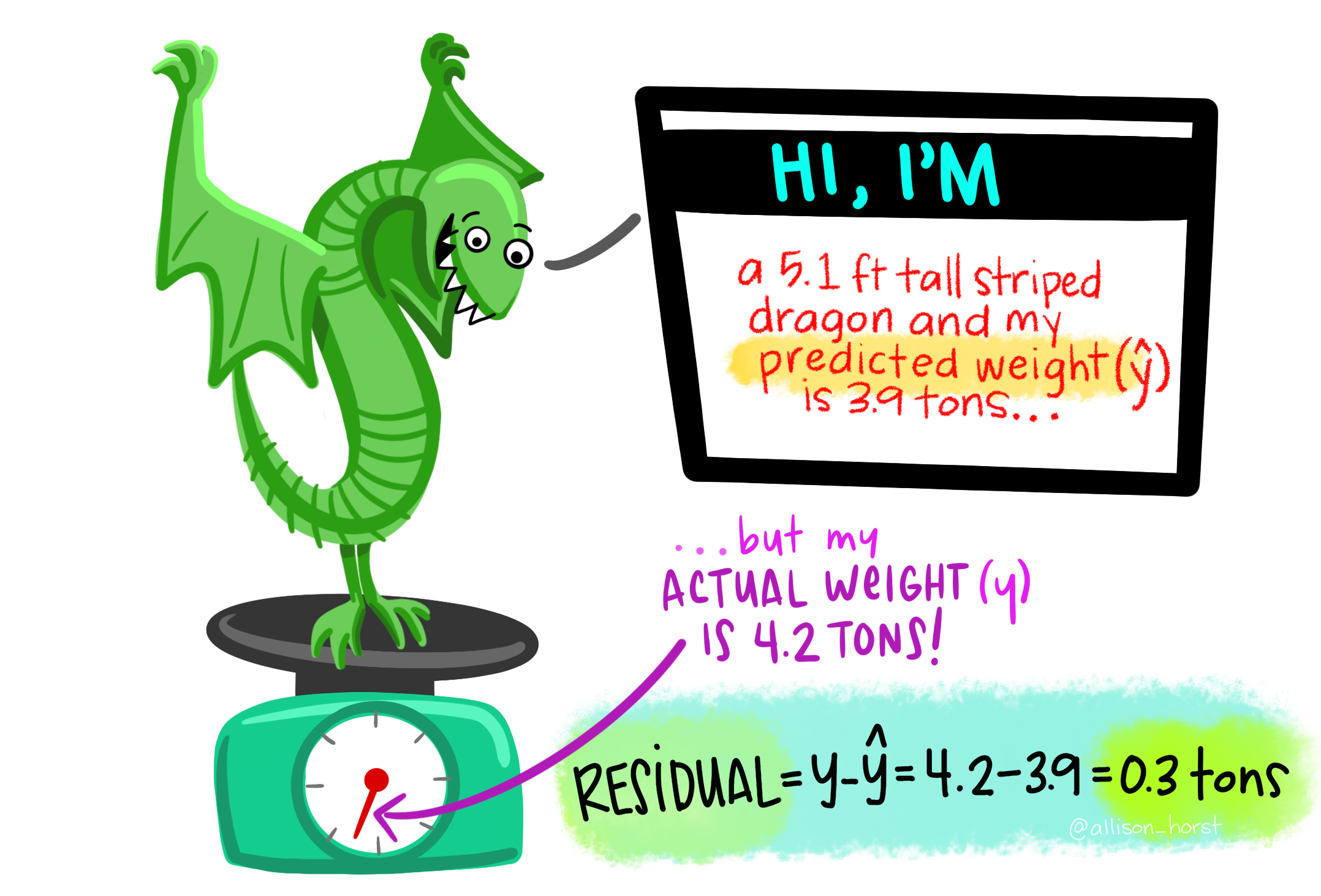
Figure 1: Recall that the residual \(e_i\) is the difference between a data point and its value predicted from a model.
Perhaps the most simple linear model is the mean. Here each individual’s predicted value is the sample mean (\(\bar{Y}\)), and the residual value is the deviation from the sample mean. So
\[Y_i = \hat{Y_i} + e_i = \bar{Y} + e_i\]
In R we use the lm() function to build linear models, with the notation \(lm(\text{response} \sim \text{explanatory}_1 + \text{explanatory}_2 + \dots, \text{data} = \text{NAMEofDATASET})\). In the case in which we only model the mean, there are no explanatory variables, so we tell R that our model is \(lm(\text{response} \sim 1)\).
Returning to our example of penguin bill length. Our model is….
lm(bill_length_mm ~ 1, data = penguins)
Call:
lm(formula = bill_length_mm ~ 1, data = penguins)

Coefficients:
(Intercept)
43.92 .](07-linear_models_files/figure-html5/meanbill-1.png)
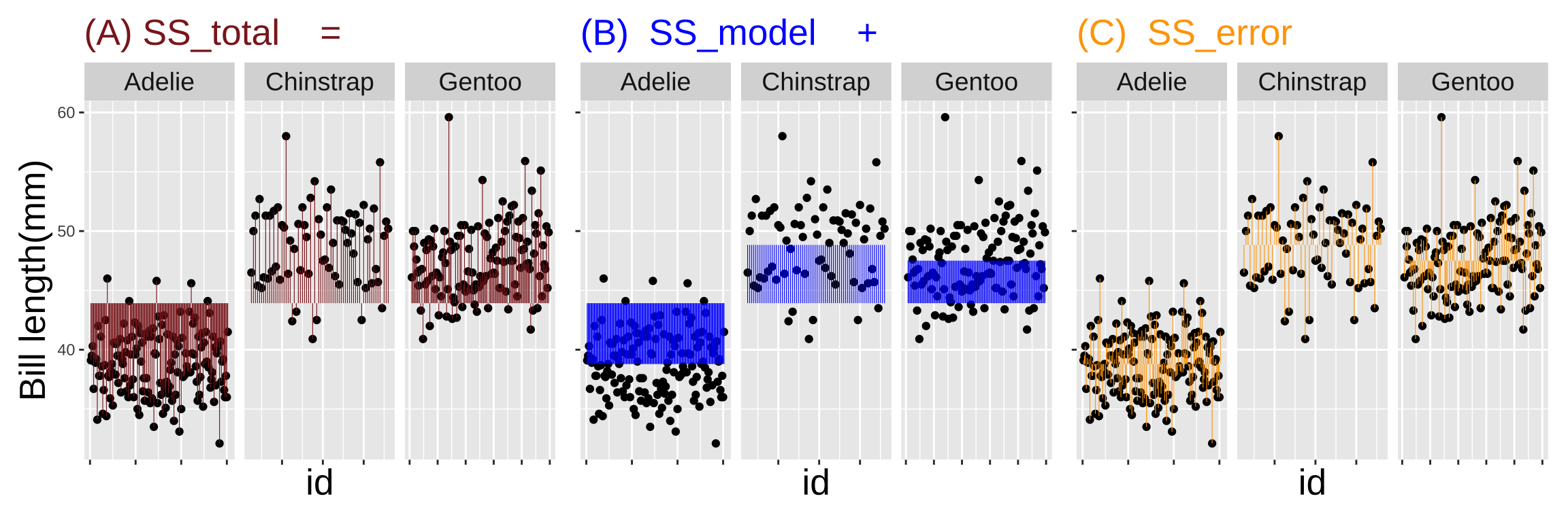
Figure 2: The mean bill length (a), Raw data with lines connecting observations to their predicted value, and (c) Residuals. The x- axis shows the order of the data in our spreadsheet code here.
Figure 2 seems a bit odd – it looks like the first half of the data is different than the second half. What could explain this difference? perhaps sex? or species? Lets have a look.
Means of two groups as a linear model.
penguins %>%  filter(!is.na(sex) & !is.na(bill_length_mm))%>% mutate(id = 1:n())%>%
  ggplot(aes(x = sex, y = bill_length_mm , color = sex))   +
  geom_boxplot()                                           +
  geom_jitter(height = 0, width = .2)                      +
  theme(legend.position = "none")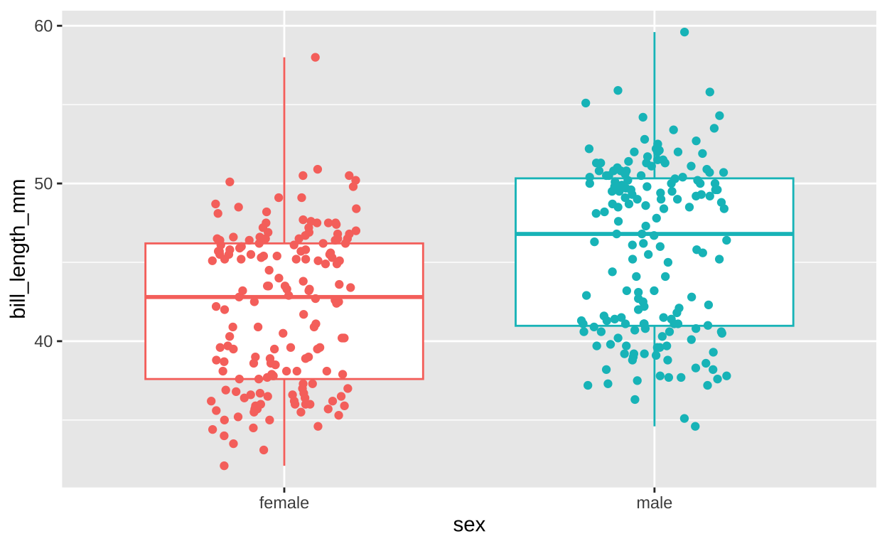
Figure 3: Sex differences in bill length.
Figure 3 totally shows a difference between bill length of male and female penguins. Again we check this out with lm(),
lm(bill_length_mm ~ sex, data = penguins)
Call:
lm(formula = bill_length_mm ~ sex, data = penguins)

Coefficients:
(Intercept)      sexmale
     42.097        3.758
As linear model now \(\text{BILL LENGTH}_i = 42.097 + 3.758 \times \text{MALE} + e_i\). This means, we start all individuals off with a BILL LENGTH of 42.097 mm, and add 3.758 mm if the penguin was a male. Reassuringly the values predicted from this model – 42.097 (for females) and 42.097 +3.758 = 45.855 (for males) – equal the means of each sex!
penguins %>%
  filter(!is.na(sex) & !is.na(bill_length_mm))%>%
  group_by(sex)%>%
  summarise(mean_bill_length_mm = mean(bill_length_mm))
# A tibble: 2 × 2
sex mean_bill_length_mm
<fct> <dbl>
1 female 42.1
2 male 45.9So that all checks out! Now lets look at our residual error and decompose this into different types of sums of squares!
penguin_SS <- penguins %>%
  filter(!is.na(sex) & !is.na(bill_length_mm)) %>%             # Remove rows with missing values for sex or bill length
  mutate(id = 1:n()) %>%                                       # Create an 'id' column to uniquely identify each row
  select(id, sex, bill_length_mm) %>%                          # Select only the necessary columns
  mutate(
    grand_mean     = mean(bill_length_mm),                     # Calculate the grand mean of bill length
    total_error    = bill_length_mm - grand_mean,              # Calculate the total deviation from the grand mean
    prediction     = 42.097 + case_when(sex == "male" ~ 3.758,
                                        sex == "female" ~ 0),  # Create predictions based on sex (simple linear model)
    model_explains = prediction - grand_mean,                  # Calculate the deviation explained by the model
    residual_error = bill_length_mm - prediction               # Calculate the residual error (unexplained by the model)
)).](07-linear_models_files/figure-html5/sssex-1.png)
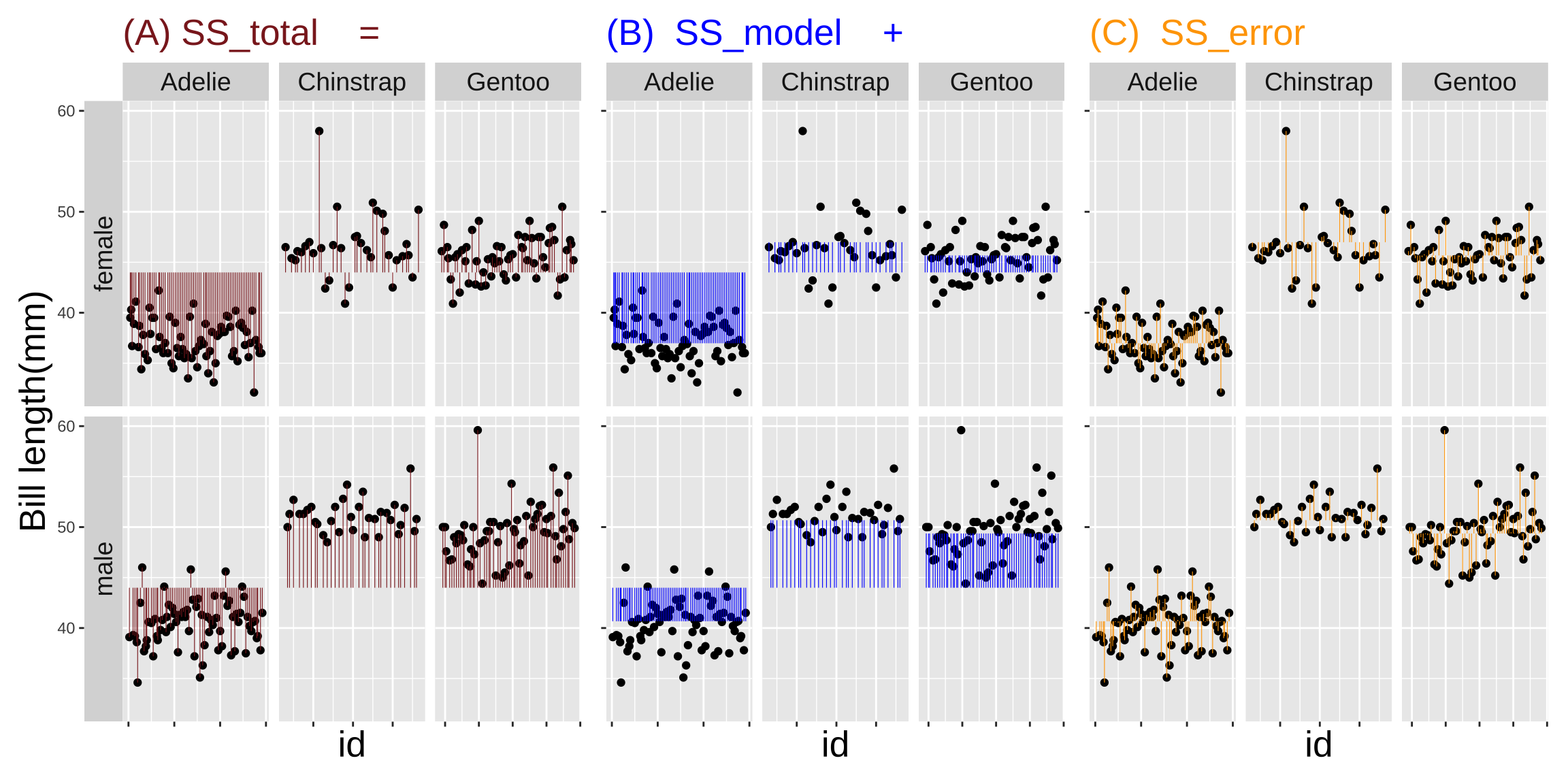
Figure 4: Partitioning the sums of squares for a model of penguin bill length as a function of sex (code here).
How much variation in bill length in these penguins is explained by sex alone? The code below calculates an \(r^2\) of 0.12.
penguin_SS %>%
  summarise(SS_total = sum(total_error^2),
            SS_model = sum(model_explains^2),
            SS_error = sum(residual_error^2),
            r2       = SS_model / SS_total)
# A tibble: 1 × 4
SS_total SS_model SS_error r2
<dbl> <dbl> <dbl> <dbl>
1 9929. 1176. 8753. 0.118Figure 4 shows that the residual variation still seems split between the first and second half ot this data set. Therefore although male penguins tend to have longer bills than female penguins – and this explains about 12% of the total variation in our sample – sex not responsible for the stark change in bill length in the second half of the data set. Now let’s look at the potential relationship between species and bill length.
Means of more than two groups as a linear model
In the previous section, we noticed a pattern in the bill lengths that seemed to differ in the first and second halves of the dataset. While sex differences explained some of the variation, they didn’t fully account for this trend. This leads us to consider another potential factor: species. Could the differences in bill length be explained by the penguin species?
Let’s first visualize the data to see if there’s an obvious difference in bill length among the species.
penguins %>%
  filter(!is.na(species) & !is.na(bill_length_mm)) %>%
  mutate(id = 1:n()) %>%
  ggplot(aes(x = species, y = bill_length_mm, color = species)) +
  geom_boxplot() +
  geom_jitter(height = 0, width = .2) +
  theme(legend.position = "none")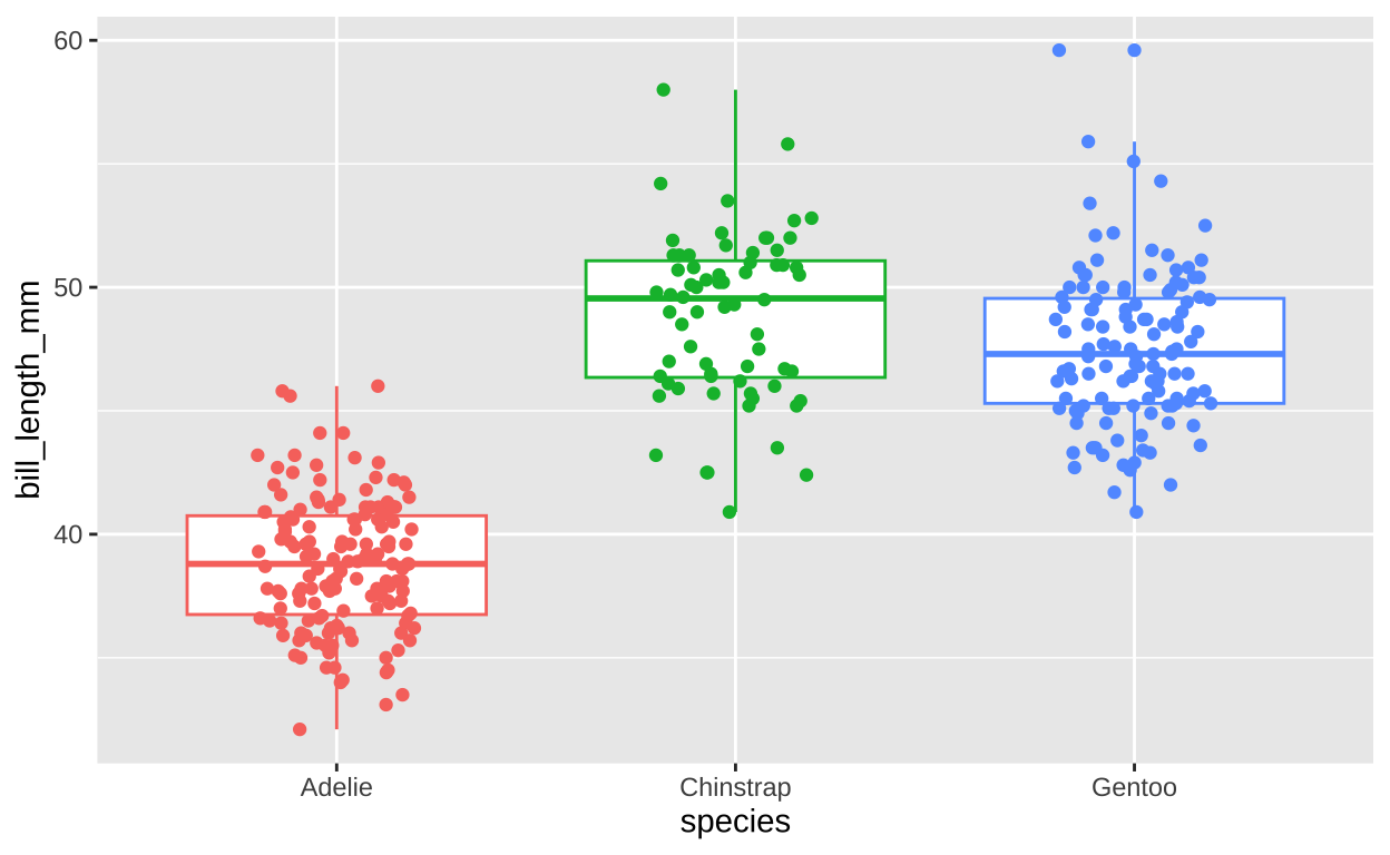
Figure 5: Species differences in bill length.
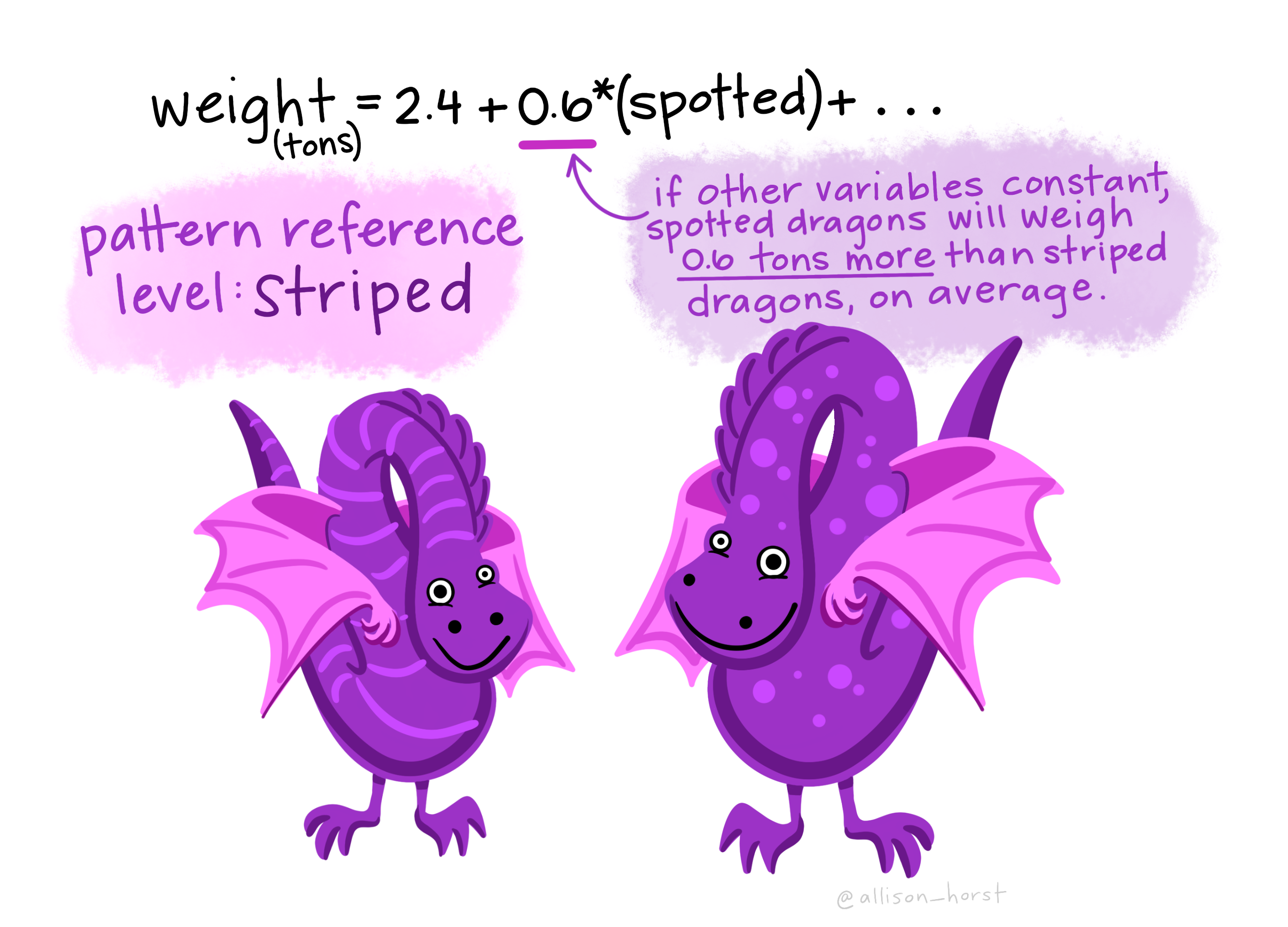
Figure 5 shows clear differences in bill length among the three species of penguins. As with a comparison between two categories, we can model mor than two categories as a linear model as well. In this case our linear model is
\[\text{BILL LENGTH}_i = \beta_0 + \beta_1 \times \text{CHINSTRAP} + \beta_2 \times \text{GENTOO} +e_i \]
were \(\beta_0\) is the reference value, \(\beta_1\) is how Chinstrap penguins differ from this reference value, and \(\beta_2\) is how Gentoo penguins differ from this reference value. What about Adelie penguins? Their predicted value is the reference value, \(\beta_0\). We can use the lm() function to find these values
lm(bill_length_mm ~ species, data = penguins)
Call:
lm(formula = bill_length_mm ~ species, data = penguins)

Coefficients:
     (Intercept)  speciesChinstrap     speciesGentoo
          38.791            10.042             8.713
Filling in these values
\[\text{BILL LENGTH}_i = 38.791 + 10.042 \times \text{CHINSTRAP} + 8.713 \times \text{GENTOO} +e_i \] So we can turn this into predictions!
- Adelie penguins have a baseline bill length of 38.791 mm.
- Chinstrap penguins have a bill length that is 10.042 mm longer than the Adelies – \(38.791 + 10.042 = 48.833\).
- Chinstrap penguins have a bill length that is 8.713 mm longer than the Adelies – \(38.791 + 8.713 = 47.504\).
Again we see that reassuringly these predictions are the species means
penguins %>%
  filter(!is.na(species) & !is.na(bill_length_mm)) %>%
  group_by(species) %>%
  summarise(mean_bill_length_mm = mean(bill_length_mm))
# A tibble: 3 × 2
species mean_bill_length_mm
<fct> <dbl>
1 Adelie 38.8
2 Chinstrap 48.8
3 Gentoo 47.5So that all checks out! Now lets look at our residual error and decompose this into different types of sums of squares! Note that rather than using case_when and manually making our predictions, I used the predict() function to do this for me.
penguin_SS_species <- penguins %>%
  filter(!is.na(species) & !is.na(bill_length_mm)) %>%
  mutate(id = 1:n()) %>%
  select(id, species, bill_length_mm) %>%
  mutate(
    grand_mean     = mean(bill_length_mm),                    # Calculate the grand mean of bill length
    total_error    = bill_length_mm - grand_mean,             # Calculate the total deviation from the grand mean
    prediction     = predict(lm(bill_length_mm ~ species, data = .)), # Predicted values from the model
    model_explains = prediction - grand_mean,                 # Deviation explained by the model
    residual_error = bill_length_mm - prediction              # Residual error
  )
How much variation in bill length in these penguins is explained by sex alone? The code below calculates an \(r^2\) of 0.71.
penguin_SS_species %>%
  summarise(SS_total = sum(total_error^2),
            SS_model = sum(model_explains^2),
            SS_error = sum(residual_error^2),
            r2       = SS_model / SS_total)
# A tibble: 1 × 4
SS_total SS_model SS_error r2
<dbl> <dbl> <dbl> <dbl>
1 10164. 7194. 2970. 0.708So we know that species – and to a lesser extent sex – can predict bill length. What if we included both in our model?
Linear models with more than one explanatory variable.
)](07-linear_models_files/figure-html5/speciessexdiff-1.png)
Figure 6: Species and sex differences in bill length. (code here)
Figure 6 shows what we’ve seen before – Adelie penguins have shorter bill than the other species and females have smaller bills than males. We can include both sex and species in the following linear model:
\[\text{BILL LENGTH}_i = \beta_0+ \beta_1 \times \text{MALE} + \beta_2 \times \text{CHINSTRAP} + \beta_3 \times \text{GENTOO} + e_i \] Here’s what the coefficients represent:
- Intercept (\(\beta_0\)): The baseline bill length for female Adelie penguins (the reference category for both sex and species).
- Sex Coefficient (\(\beta_1\)): The difference in bill length between males and females, holding species constant.
- Species Coefficients (\(\beta_2\) and \(\beta_3\)): The difference in bill length between Chinstrap and Gentoo penguins, respectively, compared to Adelie penguins.
We can use the lm() function to find these values
lm(bill_length_mm ~ sex + species, data = penguins)
Call:
lm(formula = bill_length_mm ~ sex + species, data = penguins)

Coefficients:
     (Intercept)           sexmale  speciesChinstrap
          36.977             3.694            10.010
   speciesGentoo
           8.698
Filling in these values
\[\text{BILL LENGTH}_i = 36.977 + 3.694 \times \text{MALE} + 10.01 \times \text{CHINSTRAP} + 8.698 \times \text{GENTOO} +e_i \] So we can turn this into predictions!
| female | male | |
|---|---|---|
| Adelie | 36.98 | 36.98 + 3.69 = 40.67 |
| Chinstrap | 36.98 + 10.01 = 46.99 | 36.98 + 3.69 + 10.01 = 50.68 |
| Gentoo | 36.98 + 8.70 = 45.68 | 36.98 + 3.69 + 8.70 = 49.37 |
penguins %>%
  filter(!is.na(species) & !is.na(bill_length_mm), !is.na(sex)) %>%
  mutate(prediction     = predict(lm(bill_length_mm ~ sex + species, data = .)))%>%
  group_by(species,sex) %>%
  summarise(mean_bill_length_mm = mean(bill_length_mm),
            predicted_bill_length_mm = unique(prediction))
# A tibble: 6 × 4
# Groups: species [3]
species sex mean_bill_length_mm predicted_bill_length_mm
<fct> <fct> <dbl> <dbl>
1 Adelie female 37.3 37.0
2 Adelie male 40.4 40.7
3 Chinstrap female 46.6 47.0
4 Chinstrap male 51.1 50.7
5 Gentoo female 45.6 45.7
6 Gentoo male 49.5 49.4Notice that unlike the case of one explanatory variable, with two explanatory variables predictions do not fully match means (more on that below).
How much variation in bill length in these penguins is explained by sex alone? The code below calculates an \(r^2\) of 0.82. Thus a lot of the variation in bill length in this data set is attributable to sex and species.
penguin_SS_sexspecies %>%
  summarise(SS_total = sum(total_error^2),
            SS_model = sum(model_explains^2),
            SS_error = sum(residual_error^2),
            r2       = SS_model / SS_total)
# A tibble: 1 × 4
SS_total SS_model SS_error r2
<dbl> <dbl> <dbl> <dbl>
1 9929. 8151. 1778. 0.821Models with interactions
Above, we saw that the fit between model predictions and group means was imperfect when we had two factors. This is because this model inherently assumes that the sex difference in bill length is the same across species. In this case, this assumption seems pretty close to true – so for a model this is ok. But in other cases this assumption is less justified. To allow the predicted effect of one thing to depend on another we add an interaction. This model is similar in for to the previous, buta bit more complex.
\[\begin{align} \text{BILL LENGTH}_i &= \beta_0 + \beta_1 \times \text{MALE} + \beta_2 \times \text{CHINSTRAP}+ \beta_3 \times \text{GENTOO} + \\ &\quad \beta_4 \times \text{CHINSTRAP,MALE} + \beta_5 \times \text{GENTOO,MALE} + e_i \end{align}\]
We can write our linear model in R as follows (where :specifies an interaction)
             (Intercept)                  sexmale
                    37.3                      3.1
        speciesChinstrap            speciesGentoo
                     9.3                      8.3
sexmale:speciesChinstrap    sexmale:speciesGentoo
                     1.4                      0.8
This means that e.g.to predict the bill length of a Gentoo male, we add the effect of Gentooo, the effect of Male, and the effect of GentooMale
\[\begin{align} \text{BILL LENGTH}_i &= 37.3 + 3.1 \times \text{MALE} + 9.3 \times \text{CHINSTRAP}+ 8.3 \times \text{GENTOO} + \\ &\quad 1.4 \times \text{CHINSTRAP,MALE} + 0.8 \times \text{GENTOO,MALE} + e_i \end{align}\]
| female | male | |
|---|---|---|
| Adelie | 37.3 | 37.3 + 3.1 = 40.4 |
| Chinstrap | 37.3 + 9.3 = 46.6 | 37.3 + 3.1 + 9.3 = 49.7 |
| Gentoo | 37.3 + 8.3 = 45.6 | 37.3 + 3.1 + 8.3 + 0.8 = 49.5 |
# A tibble: 6 × 4
# Groups:   species [3]
  species   sex    mean_bill_length_mm predicted_bill_length_mm
  <fct>     <fct>                <dbl>                    <dbl>
1 Adelie    female                37.3                     37.3
2 Adelie    male                  40.4                     40.4
3 Chinstrap female                46.6                     46.6
4 Chinstrap male                  51.1                     51.1
5 Gentoo    female                45.6                     45.6
6 Gentoo    male                  49.5                     49.5
Adding this interaction adds two terms to our model, and increases our \(r^2\) from 0.8209 to 0.8234. IMHO this increase hardly seems worth it in this case – but in other cases interactions can be very important.
One continuous and one categorical predictor

We first introduced linear models as regression in our section on associations, when we predicted flipper length as a function of body mass. Recall our model
length_lm <- lm( flipper_length_mm ~ body_mass_g, data = penguins)
coef(length_lm) %>% round(digits = 5)
(Intercept) body_mass_g
136.72956 0.01528 We can easily add sex as another term in our model
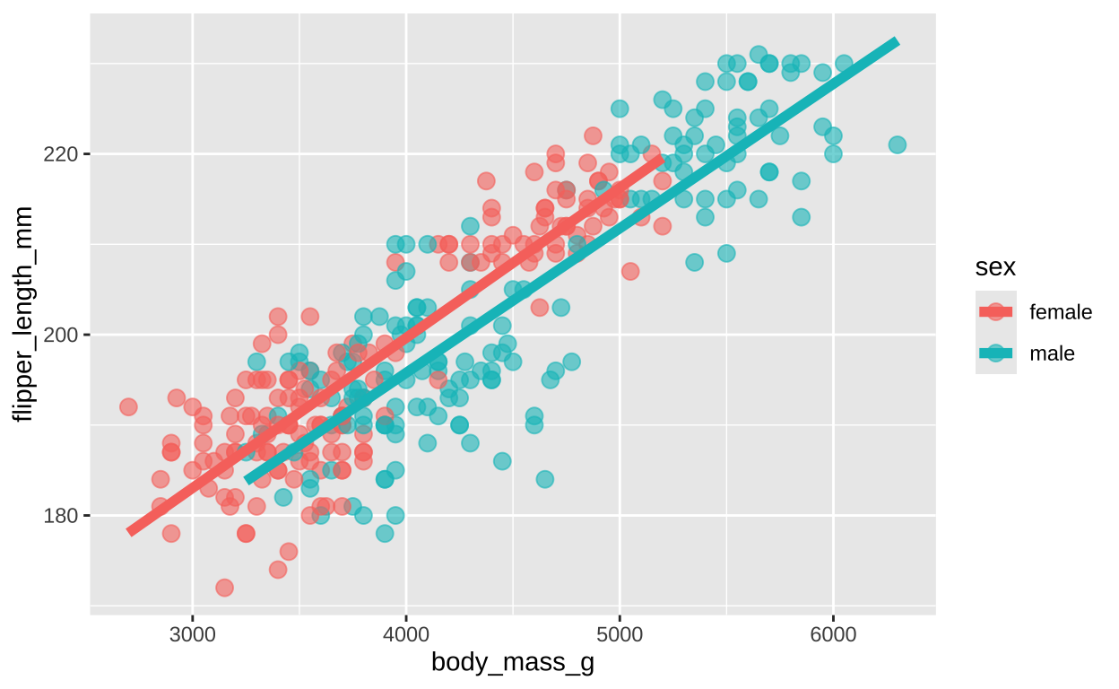
Figure 7: Flipper length as a function of sex and body mass
So now our model includes body mass and sex
\[\text{FLIPPER LENGTH}_i = \beta_0 + \beta_1 \times \text{BODY MASS} + \beta_2 \times \text{MALE} +e_i\]
Here, \(\beta_2\) represents the average difference in flipper length between males and females, holding body mass constant.
length_lm2 <- lm( flipper_length_mm ~  body_mass_g + sex, data = penguins)
coef(length_lm2) %>% round(digits = 5)
(Intercept) body_mass_g sexmale
134.63635 0.01624 -3.95700 Plugging in our values:
\[\text{FLIPPER LENGTH}_i = 134.636 + 0.016 \times \text{BODY MASS} -3.957 \times \text{MALE} +e_i\]
So returning to our 5kg penguin, we predict a flipper length of
- 134.63635 + 0.01624 = 215.8363 for a female, and
- 215.8363 - 3.95700 = 211.8793 for a male.
We can go through the procedures above to find that \(r^2 = 0.7785\).
Interactions between continuous and categorical variables.
We could even add an interaction between sex and body mass. In this case our model would be \[\text{FLIPPER LENGTH}_i = \beta_0 + \beta_1 \times \text{MALE} + \beta_2 \times \text{BODY MASS} + \beta_3 \times \text{MALE} \times \text{BODY MASS}\]
Example predictions would be
- \(\beta_0 + \beta_2 \times 6000\) for a 6kg female, and
- \(\beta_0 + \beta_1 + \beta_2 \times 6000 + \beta_3 \times 6000\) for a 6 kg male.
In this example too, it seems like the interaction term is not particularly meaningful. This is revealed in Figure 8 To see this, I will plot predicted values from each model against one another
penguins %>%
  filter(!is.na(sex))%>%
  mutate(predict_no_interaction = predict(lm(flipper_length_mm ~  sex + body_mass_g, data = .)),
         predict_with_interaction = predict(lm(flipper_length_mm ~  sex + body_mass_g + sex : body_mass_g, data = .))) %>%
  ggplot(aes(x = predict_no_interaction , y = predict_with_interaction, color = sex))+
  geom_point(size = 3, alpha = .2)+
  geom_smooth(method = "lm", se = FALSE)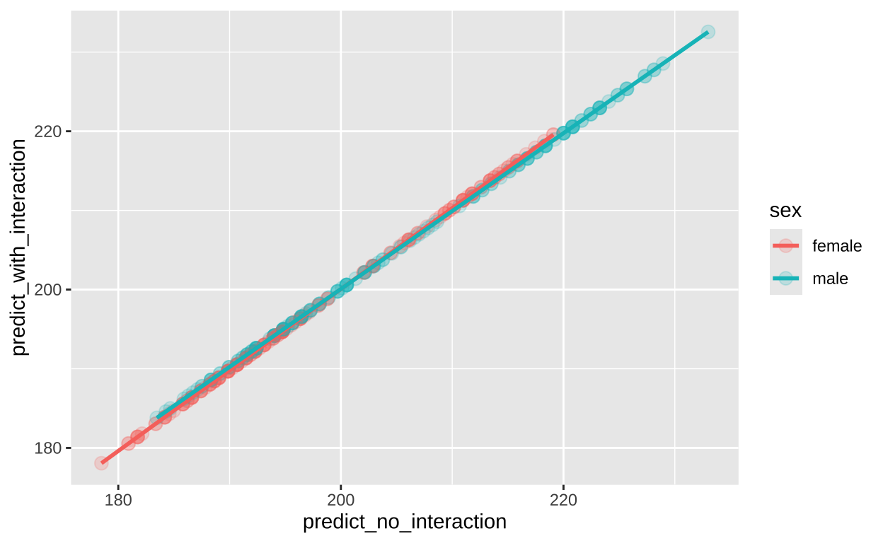
Figure 8: Predicted flipper length as a function of sex and body mass for models with (y-axis) and without (x-axis) an interaction between explanatory variables.
Additional notes on linear models:
Interactive efects
The fitness at a single locus ripped from its interactive context is about as relevant to real problems of evolutionary genetics as the study of the psychology of individuals isolated from their social context is to an understanding of man’s sociopolitical evolution. In both cases context and interaction are not simply second-order effects to be superimposed on a primary monadic analysis. Context and interaction are of the essence.
Page 318 of “The genetic basis of evolutionary change” – Richard Lewontin (1974)
Above I showed that we can include an interaction between variables in R with the syntax var1:var2, and I showed you how to make predictions from interactions. But neither example actually showed an interesting interaction. This is too bad because, as Lewontin frocefully argrued, interactions are very important across life.
Visualizing interactions
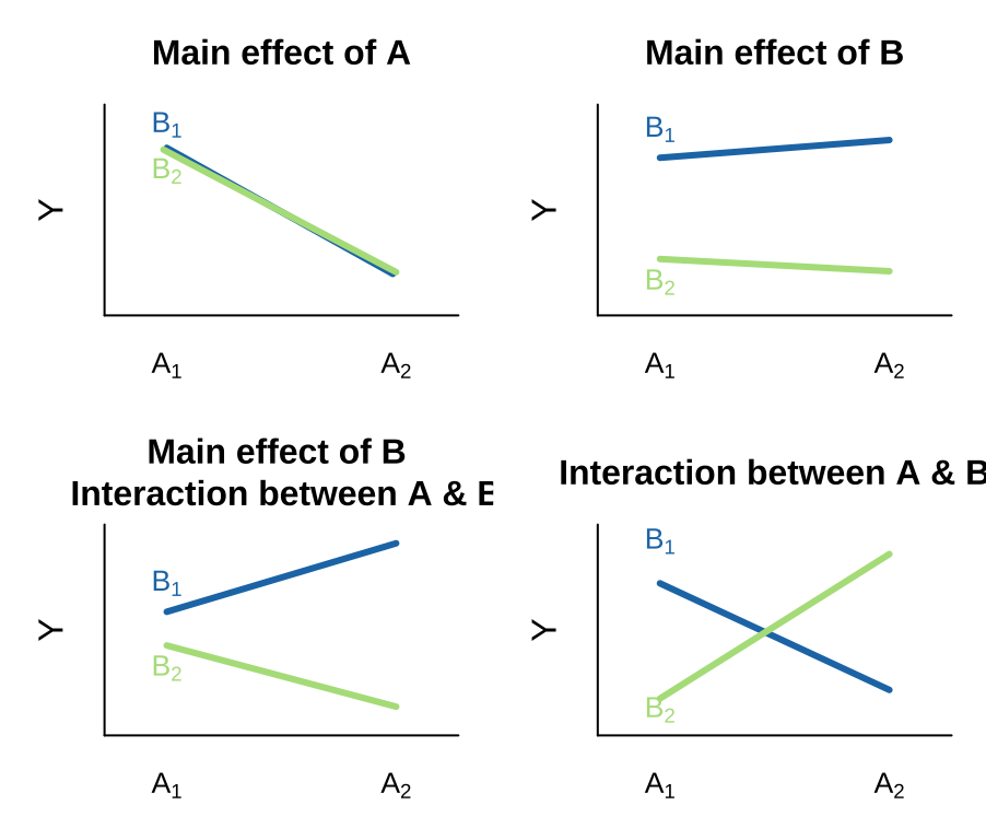
There are many possible outcomes when looking into a model with two predictors and the potential for an interaction. I outline a few extreme possibilities, plotted on the right.
- We can see an effect of only variable A on Y. That is, lines can have nonzero slopes (“Main effect of A”).
- We can see a effect of only variable B on Y. That is, lines can have zero slopes but differing intercepts (“Main effect of B”).
- We can see an effect of only variable B on Y, but an interaction between that variable and the other. That is, intercepts and slopes can differ (or vice versa) in such a way that the mean of Y only differs by one of the explanatory variables (e.g. “Main effect of B, Interaction between A & B”). and/or
- We can have only an interaction. That is, on their own values of A or B have no predictive power, but together they do. (different slopes)
Simple interaction example
Take, for example, the interaction between toothpaste and orange juice I like orange juice in the morning. I also like the taste of minty fresh toothpaste. But drinking orange juice after brushing my teeth tastes terrible. Here the chemical Sodium lauryl sulfate (SLS) found in toothpaste suppresses the sweet receptors in our taste buds, leaving only the bitter flavor for us to pick up. This is an example of an interaction.
- On its own, toothpaste tastes good.
- On its own OJ is even better.
- Put them together, and you have something gross.

This is an extreme case. More broadly, an interaction is any case in which the slope of two lines differ – that is to say when the effect of one variable on an outcome depends on the value of another variable.
Caution in interpreting \(r^2\)
We refer to $r^2 as the “proportion variance explained.” However, it is more approriate to call \(r^2\) “the proportion variance explained in this study.”
WARNING: While \(r^2\) is a nice summary of the effect size in a given study, it cannot be extrapolated to beyond that experiment. Importantly \(r^2\) depends on the relative size of each sample, and the factors they experience.
- It’s WRONG to say Together sex and species explain 82 percent of variation in penguin bill length.
- It’s RIGHT to say Together sex and species explain 82 percent of variation in penguin bill length in this study.
What makes a good linear model?
A linear model is a description of data… but some descriptions are more useful than others. A good linear model has the following features.
It captures the essence of the biological system – the descriptors should focus on the key bits likely important for the system. This means including predictors that are known or hypothesized to have a biological relevance or impact on the response variable.
It generalizes well to new, unseen data. It should capture the underlying pattern without being overly tailored to the specific dataset – that is, be careful not to “overfit” our model. Our goals is to provide a clean description, not to maximize \(r^\). Overfitting happens when the model includes too many predictors or overly complex relationships, making it fit the specific dataset too closely and not generalize to new data. Later in the term we will look into how leave-one-out and other cross-validation approaches can be used to asses a model by testing it on subsets of the data it wasn’t trained on.”
It explains most of the data equally well. That is, we don’t want a linear model that e.g. explains large values of the response variable well, but does a poor job explaining small values.
It is simple and interpretable: The model should be straightforward enough to interpret easily while still capturing the essential relationships in the data. A simpler model provides clearer insights into the data without overcomplicating the interpretation.
Quiz
Figure 9: The accompanying quiz link