Chapter 15: Uncertainty

Communicating our skepticism in the preceision of our estimates

If you want a different (or another) presentation of this material, I highly recommend Chapter 8 of Ismay and Kim (2019) as an optional reading.

If you want to read more about visualizing uncertainty, I suggest Clause Wilke’s chapter on the subject (Wilke 2019). I also suggest this article from Nature Methods

Motivating scenarios: You have a sample and made an estimate, and want to communicate the precision of this estimate.

Learning goals: By the end of this chapter you should be able to:

• Explain why the idea of the sampling distribution is useful in communicating our uncertainty in an estimate.
  
• Describe the challenge we have in building a sampling distribution from a single sample.
  
• Explain how we can build estimate a sampling distribution from a single sample by resampling with replacement.
  
• Use R to bootstrap real data.
  
• Describe the concept of the confidence interval.
  
• Calculate bootstrapped standard errors and bootstrapped confidence intervals.
  
• Recognize why/when we would (or would not) use the bootstrap to quantify uncertainty.
  
• Know how to visualize uncertainty in R.

In addition to this reading, the other assignments are:

• Take a single bootstrap (described below)
  
• Watch from 0:54 to 3:32, plus 4:53 to 6:49, and 10:50-12:20 from this Crash Course Statistics video about confidence intervals (split into three below).
  
• Explore the webapp about confidence intervals, below.
  
• Complete the uncertainty quiz below and finish on canvas.

Review: We estimate population parameters from samples.

In the section on sampling we sampled from a population many times to build a sampling distribution. But, if we had data for an entire population, we would know population parameters, so there would be no reason to calculate estimates from a sample.

In the real world we have a small number (usually one) of sample(s) and we want to learn about the population. This is a major a major challenge of statistics (See our Introduction Statistics).

Review: Populations have parameters

We conceptualize populations as truth with true parameters out there.

Review: Sampling involves chance

Because (a good) sample is taken from a population at random, a sample estimate is influenced by chance.

Review: The standard error

The sampling distribution – a histogram of sample estimates we would get by repeatedly sampling from a population – allows us to think about the chance deviation between a sample estimate and population parameter induced by sampling error.

The standard error quantifies this variability as the standard deviation of the sampling distribution.

Reflect on the two paragraphs above. They contain stats words and concepts that are the foundation of what we are doing here.

• Would this have made sense to you before the term?
  
• Does it make sense now? If not, take a moment, talk to a friend, email Yaniv or Anna, whatever you need. This is important stuff and should not be glossed over.

Estimation with uncertainty

Because estimates from samples take their values by chance, it is irresponsible and misleading to present an estimate without describing our uncertainty in it, by reporting the standard error or other measures of uncertainty.

Generating a sampling distribution

Question: We usually have one sample, not a population, so how do we generate a sampling distribution?
Answer: With our imagination!!! (Figure 1).

What tools can our imagination access?

• We can use math tricks that allow us to connect the variability in our sample to the uncertainty in our estimate.
  
• We can simulate the process that we think generated our data.
  
• We can resample from our sample by bootstrapping (describe below).

Figure 1: We use our imagination to build a sampling distribution by math, simulation, or bootstrapping.

Don’t worry about the first two too much – we revisit them throughout the course. For now, just know that whenever you see this, we are imagining an appropriate sampling distribution. Here we focus on bootstrapping.

Resampling from our sample (Bootstrapping)

While statistics offers no magic pill for quantitative scientific investigations, the bootstrap is the best statistical pain reliever ever produced.

— Xiao-Li Meng

As quoted in Cochran (2019)

So we only have one sample but we need to imagine resampling from a population. One approach to build a sampling distribution in this situation is to assume that your sample is a reasonable stand-in for the population and resample from it.

Of course, if you just put all your observed values down and picked them back up, you would get the same estimate as before. So we resample with replacement and make an estimate from this resample – that is, we

1. Pick an observation from your sample at random.
   
2. Note its value.
   
3. Put it back in the pool.
   
4. Go back to (1) until you have as many resampled observations as initial observations.
   
5. Calculate an estimate from this collection of observations.
   
6. After completing this you have one bootstrap replicate.

Optional Exercise: Physically generate a bootstrap replicate. We will soon learn how to conduct a bootstrap in R, but I find that getting physical helps it all be real, and gives us more appreciation for what is going on in a bootstrap. So, our assignment is to generate a single bootstrap replicate by brute force

1. Find a sample of about twenty of something that is easy to quantify, I suggest the date on n = twenty pennies if you have them. If all else fails you can write down values on a piece of paper (e.g. the point differential for Timberwolves games this season, the length of twenty songs on your itunes etc..)
   
2. Estimate the sample mean (i.e. What is the mean date of issue of pennies in your sample).
   
3. Shove your observations in a bag or sock or something.
   
4. Generate an estimate from a single bootstrap replicate. Sample n observations with replacement, and calculate your estimate from this bootstrap replicate.

To get the bootstrapped sampling distribution, you would repeat this process many times, but that is too tedious to do manually. For now, try to imagine what would happen.

While the exercise above was useful, it would be tedious and unfeasible to do this more than a handful of times. Luckily, we don’t have to, we can use a computer to conduct a bootstrap.

Bootstrapping computation and example.

EXAMPLE Let’s stick to our penguins example, but to make it all easier to follow, let’s just focus on female Chinstrap penguins. We use the filter() function in dplyr to reduce our penguins data set down to only Chinstrap females. We will also add an id column with mutate(), and select() only the id and bill_length_mm columns to make the data easier to deal with (we don’t need sex or species because we only have chinstrap females).

chinstrap_females <- penguins %>%
  dplyr::filter(species == "Chinstrap" , sex == "female") %>%
  dplyr::mutate(id = factor(1:n())) %>%
  dplyr::select(id, bill_length_mm)

First (as always) let’s look at the actual data. You could do this with glimpse(), view(), or just typing firefly.

Calculating estimates from the data

Next we get our basic data summaries (note, that I am calculating variances and standard deviation with math instead of with the var() and sd()) functions. This is to help us remember the underlying calculation. eel free to avoid this extra work ;) ). We can bootstrap any estimate - a mean, a standard deviation, a median, a correlation, an F statistic, a phylogeny, whatever. But we will focus on themean for simplicity.

chinstrap_females %>%
  summarize(mean_bill_length   = mean(bill_length_mm, na.rm = TRUE),
            median_bill_length = median(bill_length_mm, na.rm = TRUE),
            var_bill_length    = sum((bill_length_mm - mean_bill_length)^2,na.rm = TRUE)/(n()-1),
            sd_bill_length     = sqrt(var_bill_length)) %>%
  mutate_all(round, digits = 2)

# A tibble: 1 × 4
  mean_bill_length median_bill_length var_bill_length sd_bill_length
             <dbl>              <dbl>           <dbl>          <dbl>
1             46.6               46.3            9.66           3.11

So, our sample estimate is that the mean bill length of a female chinstrap penguin is 46.57. But that is just our sample. It could have been different if we had different penguins! So, we cannot learn the true population parameter, but we can bootstrap to get a sense of how far from the true parameter we expect an estimate to lie.

Resampling our data (with replacement) to generate a single bootstrap replicate

First, let’s use the slice_sample() function to generate a sample of the same size. You will notice that this code is very similar to what we wrote for sampling except that we

1. Sample with replacement – that is, we tell R to toss each observation back and mix up the bag every time, outlined in above.
   
2. Take a (resampled) sample that is the same size as our sample, rather than a subsample of our population.

# One bootstrap replicate  
resampled_chinstrap_females <- chinstrap_females  %>%         
  slice_sample(prop = 1, replace = TRUE) # resample the data with replacement

So, lets look at the resampled data:

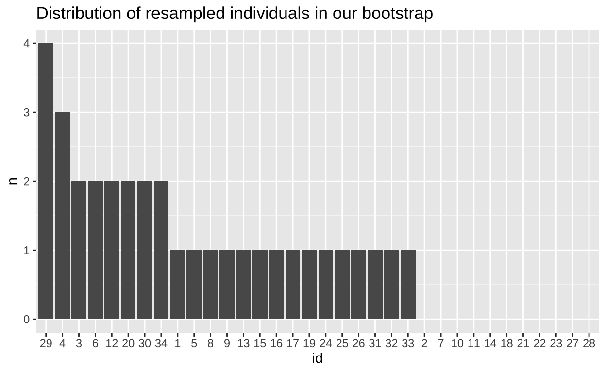
To confirm that my resampling with replacement worked, let’s make sure some we see some individuals more than once, and some not at all. To do so, I present a simple plot showing the number of times each individual was sampled. Note that some are not sampled at all while some are sampled two, three, four, or more times!

Now that it looks like we resampled with replacement correctly, let’s make an estimate from this resampled data.

resampled_chinstrap_females %>%
  summarize(mean_bill_length   = mean(bill_length_mm, na.rm = TRUE))

# A tibble: 1 × 1
  mean_bill_length
             <dbl>
1             45.8

So, the difference between the sample estimate and the resample-based estimate is 0.81. But this is just one bootstrap replicate.

Resampling many times to generate a bootstrap distribution

Let’s do this many (10,000) times with the replicate() function, much like we did previously with repeated sampling to generate a sampling distribution – except we set prop = 1 and replace = TRUE (rather than size = sample.size - were is sample.size\(<\) population.size, and replace = FALSE). The analogy to repeated sampling helps us see what we are trying to do – we don’t have a population o repeatedly sample from, but we use our sample as a stand in for a population to estimate the sampling distribution. We then visualize this bootstrapped sampling distribution as a histogram.

sample_estimate  <- chinstrap_females %>%
  summarise(mean(bill_length_mm, na.rm = TRUE)) %>%
  pull()

n_boots <- 10000

bill_length_mm_boot <- replicate(n = n_boots, simplify = FALSE,              # tell R to do this a bunch, and to keep each result as its own tibble
    expr = slice_sample(chinstrap_females, prop =  1, replace = TRUE) %>%    # same code as above
    summarise(boot_mean_bill_length = mean(bill_length_mm)))        %>%      # calculate proportion with mean()
  bind_rows()      


boot_dist_plot <- ggplot(bill_length_mm_boot, aes(x = boot_mean_bill_length)) +   # assign plot to a variable
  geom_histogram(fill = "firebrick", color = "white", bins=40)+
  geom_vline(xintercept = sample_estimate, lty = 2)+ # add a line to show the sample estimate   
  labs(title = "The bootstrapped sampling\ndistribution",
       subtitle = "Bill lengths of female chinstrao penguins (in mm, n = 34).")

boot_dist_plot  ## show the plot

Figure 2: The bootstrapped sampling distribution. Dashed line represents sample estimate.

AWESOME! So what happened here? We had a sample, not a population. but we resampled from it with replacement to generate a sampling distribution. This histogram depicts the expected sampling error from a population that resampled our sample. So we can use this to get a sense of the expected sampling error in our actual population which we do not explore beyond this sample.

Note that this is a good guide - but is not foolproof. Because we start with a sample from the population, this bootstrapped sampling distribution, will differ from our population sampling distribution – but it is a reasonable estimate!!!

Bootstrapping: Notes and considerations

The bootstrap is incredibly versatile - it can be used for any estimate, and, with enough care for study design, can be applied to almost any statistical problem. Because the bootstrap does not assume much about the shape of the variability in a population, it can be used when many other method we cover this term fail.

Because it requires some computer skills, and because it solves hard problems, the bootstrap is often taught at the end of an intro stats course. For example, the bootstrap is covered in Computer intensive methods (Section 19.2) of Whitlock and Schluter (2020). But I introduce it early because it is both useful and helps us think about the sample standard error and confidence intervals (below).

If you don’t know anything about statistics, learn the bootstrap. Seriously, think of it as a “statistical pain reliever”!! My new favorite term for the approach that underlies almost everything I do... https://t.co/jCHozq80oM

— Ryan Hernandez (@rdhernand) March 9, 2019

That said, a bootstrap is not always the best answer.

• Bootstrapping requires a reasonable sample size, such that the breadth of values in the population is sampled [as a thought experiment, imagine bootstrapping with one or two observations – the answer would clearly be nonsense]. The minimum sample size needed depends on details of the population distribution etc.., but in many cases a sample of size twenty is large enough for bootstrapping to be reasonable.

• Because a bootstrap depends on chance sampling, it will give (very slightly) different answers each time. This can be frustrating.

The bootstrap method described above is known more formally as the empirical bootstrap. Parametric bootstrapping – in which we estimate parameters and use them to simulate a sampling distribution – represent a different way to generate a sampling distribution.

Estimating the standard error

In Section the Sampling section we learned how to generate a (potentially infinite) number of samples of some size from a population to calculate the true standard error. But, in the real world we estimate the standard error from a single sample. Again, we can use our imagination to calculate the standard error, and again we have math, simulation, and resampling as our tools.

The bootstrap standard error

Here, we focus on the bootstrap standard error as an estimate of the standard error. Because the standard error measures the expected variability among samples from a population as the standard deviation of the sampling distribution, the bootstrap standard error estimates the standard error as the standard deviation of the bootstrapped distribution.

We already did the hard work of bootstrapping, so now we find the bootstrap standard error as the standard deviation of the bootstrapped sampling distribution.

chinstrap_female_bill_length_boot_SE <- bill_length_mm_boot %>% 
  summarise(SE = sd(boot_mean_bill_length))

chinstrap_female_bill_length_boot_SE %>% round(digits = 3)

# A tibble: 1 × 1
     SE
  <dbl>
1 0.526

What is the difference between the bootstrap standard error described here and and standard error in the Sampling Section?

• With sampling we (1) take many samples from our population, (2) summarize them to find the sampling distribution, and (3) take the standard deviation of these estimates to find the population standard error.

• In bootstrapping, we (1) resample our sample many times, (2) summarize these resamples to approximate (a.k.a. fake) a sampling distribution, and (3) take the standard deviation of these estimates to estimate the standard error as the bootstrap standard error.

Confidence intervals

Watch the videos below for a nice explanation of confidence intervals. Note: I split this video into three parts and excluded the bits about the mathematical calculation of confidence intervals for data from the binomial and normal distributions as those are distractions at this point. We will return to calculations as they arise, but for now we will estimate confidence intervals by bootstrapping.

part 1

Figure 3: Explanation of confidence intervals from Crash Course Statistics. I split this into three parts removing the bits that are not immediately relevant to us.

part 2

part 3

As explained in the videos above, Confidence intervals provide another way we describe uncertainty. To do so we agree on some level of confidence to report, with 95% confidence as a common convention.

Confidence intervals are a bit tricky to think and talk about. I think about a confidence interval as a net that does or does not catch the true population parameter. If we set a 95% confidence level, we expect ninety five of every one hundred 95% confidence intervals to capture the true population parameter.

Explore the webapp from Whitlock and Schluter (2020) to make this idea of a confidence interval more concrete. Try changing the sample size (\(n\)), population mean (\(\mu\)), and population standard deviation (\(\sigma\)), to see how these variables change our expected confidence intervals.

Figure 4: Webapp from Whitlock and Schluter (2020) showing the distribution of confidence intervals. Find it on their website.

Because each confidence interval does or does not capture the true population parameter, it is wrong to say that a given confidence interval has a given chance of catching the parameter. The parameter is fixed, it is the chance sampling of the sample from which we calculate the confidence interval where the chance happens.

So, how do we calculate confidence intervals? Like the standard error, we can calculate confidence intervals with math, simulation or resampling. We explore the other options in future Sections, but discuss the bootstrap based confidence interval here.

The bootstrap confidence interval

We can estimate a specified confidence interval as the middle region consisting of that proportion of bootstrap replicates. So the edges between the middle 95% of bootstrap replicates and more extreme resamples denote the 95% confidence interval. We can use the quantile() function in R to find these breaks of the bootstrap.

chinstrap_female_bill_length_boot_CI <- bill_length_mm_boot %>% 
  reframe(CI               = c("lower 95", 'upper 95'), # add a column to note which CIs we're calculating
          mean_bill_length = quantile(boot_mean_bill_length,probs = c(.025,.975)))  # boundaries separating the middle 95% from the rest of our bootstrap replicates. 

chinstrap_female_bill_length_boot_CI 

# A tibble: 2 × 2
  CI       mean_bill_length
  <chr>               <dbl>
1 lower 95             45.6
2 upper 95             47.6

So we are 95% confident that the true mean is between 45.59 and 47.65.

A confidence interval should be taken as a guide, not a bright line. There is nothing that magically makes 47.55 a plausible value for the mean and 47.75 implausible.

Visualizing uncertainty

In addition to stating our uncertainty in words, we should show our uncertainty in plots. The most common display of uncertainty in a plot is the 95% confidence interval, but be careful, and clear, because some people report standard error bars instead of confidence intervals (and others display measures of variability rather than uncertainty).

We can add these confidence intervals to our plot to show this uncertainty.

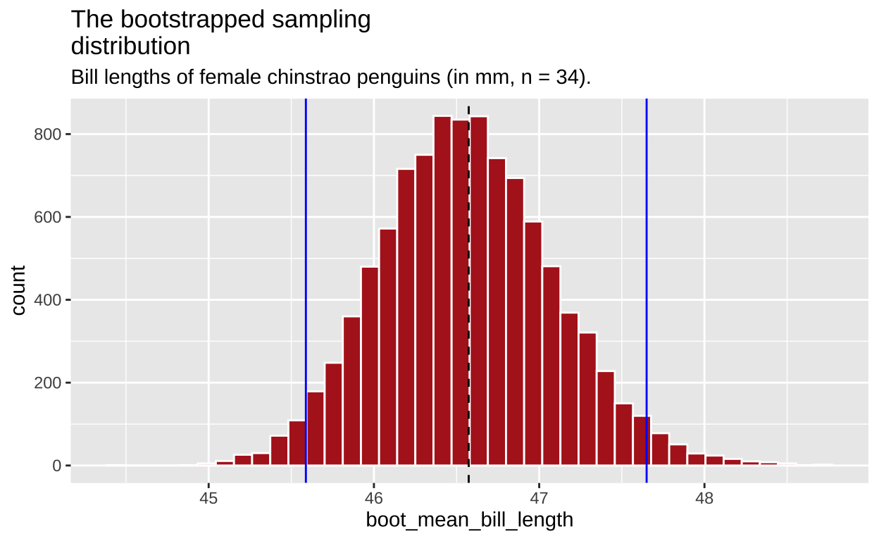
Figure 5: The bootstrapped sampling distribution. Dashed black line represents sample estimate. Dotted blue line shows 95% confidence limits.

But we almost never show the bootstrap distribution – because it not interesting. More often we show the actual data plus 95% confidence intervals (generated by bootstrap or some other method).

While this display is most traditional Clause Wilke has recently developed a bunch of fun new approaches to visualize uncertainty (see his R package, ungeviz), and the chapter on the subject (Wilke 2019), is very fun. We show one such sample in Figure 6.

Figure 6: A novel form of visualizing uncertainty provides a smoother view of uncertainty, to complement the traditional confidence limits based display.

Common mathematical rules of thumb

So long as a sample isn’t too small, the bootstrap standard error and bootstrap confidence intervals are reasonable descriptions of uncertainty in our estimates.

Above, we also pointed to mathematical summaries of uncertainty. Throughout the term, we will cover different formulas for the standard error and 95% confidence interval, which depends on aspects of the data – but rough rules of thumb are:

• For normally distributed data the standard error (aka the standard deviation of the sampling distribution) equals the standard deviation divided by the square root of the sample size, so we often approximate the sample standard error as \(SE_x = \frac{s_x}{\sqrt{n}}\).
  
• The 95% confidence interval is approximately the mean plus or minus two times the standard error.

Uncertainty Quiz

Figure 7: The accompanying uncertainty quiz link.