Motivating Scenario:
Suppose you’re interested in investigating the effects of two different factors on a biological outcome. For example, you might examine the influence of fertilizer type and watering frequency on plant growth. Or perhaps you’re curious about how different diets and exercise routines affect body weight across various age groups. Each of these cases involves multiple groups, but importantly, also more than one factor. With a two-way ANOVA, we can analyze the main effects of each factor and their interaction, answering questions such as whether the combined effect of fertilizer and water is greater than each factor alone.
Learning Goals: By the end of this chapter, you should be able to:
- Explain why multiple factors are analyzed together rather than independently.
- Describe and interpret main effects and interaction effects.
- Identify and calculate different “sums of squares” visually and mathematically.
- Calculate an F-statistic for both main and interaction effects and interpret results.
- Perform a two-way ANOVA in R and conduct post-hoc tests for further analysis.
Review of Linear Models
A linear model predicts the response variable, as \(\widehat{Y_i}\) by adding up all components of the model.
\[\begin{equation} \hat{Y_i} = a + b_1 y_{1,i} + b_2 y_{2,i} + \dots{} \tag{1} \end{equation}\]
Linear models we have seen
- One sample t-tests: \(\widehat{Y} = \mu\)
- Two sample t-tests: \(\widehat{Y_i} = \mu + A_i\) (\(A_i\) can take 1 of 2 values)
- ANOVA: \(\widehat{Y_i} = \mu + A_i\) (\(A_i\) can take one of more than two values)
- Regression \(\widehat{Y_i} = \mu + X_i\) (\(X_i\) is continuous)
Test statistics for a linear model
- The \(t\) value describes how many standard errors an estimate is from its null value.
- The \(F\) value quantifies the ratio of variation in a response variable associated with a focal explanatory variable (\(MS_{model}\)), relative to the variation that is not attributable to this variable (\(MS_{error}\)).
The two way ANOVA as a linear model
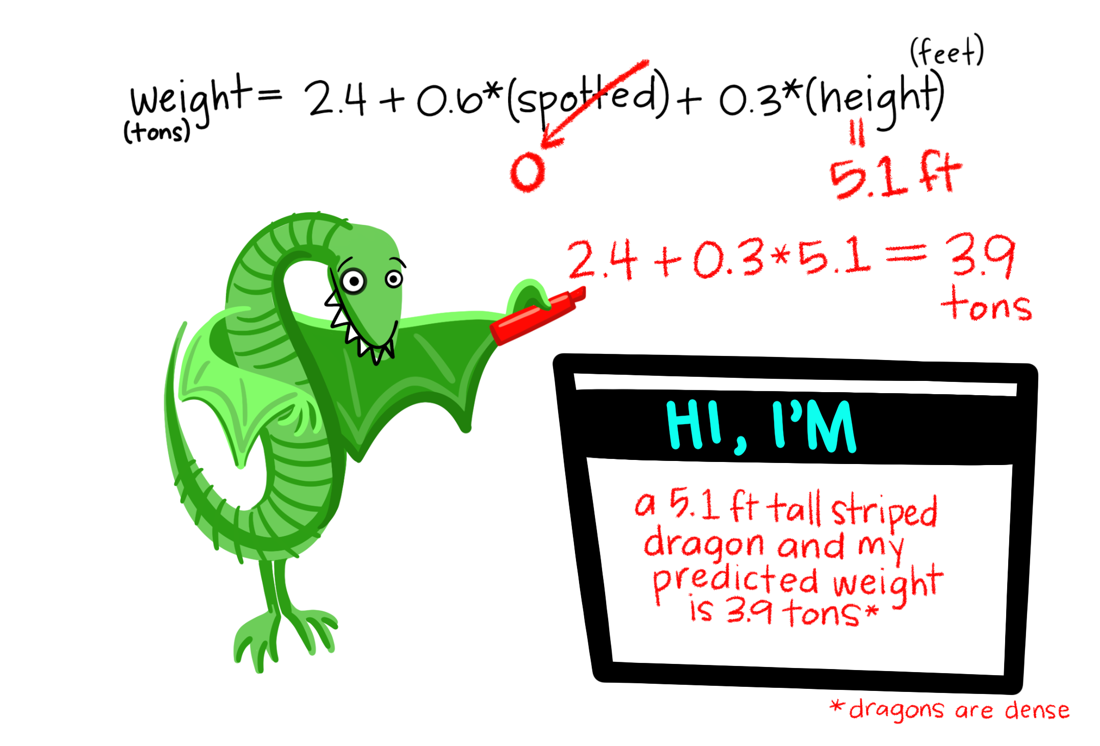
So far we’ve mainly modeled a continuous response variable as a function of one explanatory variable. But linear models can include multiple predictors – for example, we can predict Dragon Weight as a function of two categorical (e.g. spotted: yes/no, and color: green/purple/blue) and variables in the same model. Here
\[\text{WEIGHT}_i = f(\text{SPOTTED}\text{COLOR})\] \[\hat{Y_i} = a + \text{SPOTTED} \times b_\text{ SPOTTED} + \text{PURPLE} \times b_\text{ PURPLE} + \text{BLUE} \times b_\text{ BLUE}\]
We can even include an interaction such that effect of spottedness on weight depends on color (more on that later)
Two-Way ANOVA Example
In the study below, researchers investigated whether the presence of a fish predator influenced marine zooplankton diversity in a particular area. To test this, they introduced three levels of “treatment”—zooplankton exposed to no fish, some fish, or a high density of fish—contained within mesh bags in a stream. Each stream received all three treatments: one bag with no fish, another with some fish, and a third with many fish. This setup was replicated across five streams, making each stream a “Block.”
The experiment exemplifies a randomized “Controlled Blocked Design.” In this design, each “block” receives all treatments, allowing us to account for block-specific variability unrelated to our main question. Here, the block effect itself isn’t of interest, but including it in the model helps us explain additional variation before focusing on the treatment effect.
The raw data is shown below, with treatment means in the final column.
zoo_link <- "https://whitlockschluter3e.zoology.ubc.ca/Data/chapter18/chap18e2ZooplanktonDepredation.csv"
zoo <- read_csv(zoo_link) %>%
  mutate(treatment = fct_relevel(treatment, c("control", "low", "high"))) %>% # Set control as first, high as last
  mutate(block = factor(block)) # Specify block as categorical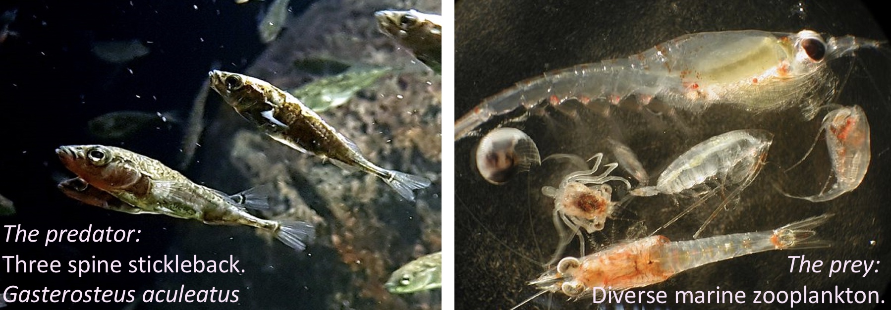
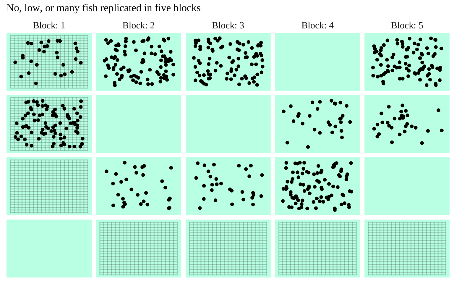
Figure 1: The prey with none, some, or many predators in mesh bags across five streams
| treatment | Block: 1 | Block: 2 | Block: 3 | Block: 4 | Block: 5 | mean_diversity |
|---|---|---|---|---|---|---|
| control | 4.1 | 3.2 | 3.0 | 2.3 | 2.5 | 3.02 |
| low | 2.2 | 2.4 | 1.5 | 1.3 | 2.6 | 2.00 |
| high | 1.3 | 2.0 | 1.0 | 1.0 | 1.6 | 1.38 |
Why Not Two Separate ANOVAs?
One might consider running two separate ANOVAs:
- One to test the relationship between block and zooplankton diversity
- Another to test the relationship between treatment (fish predator density) and zooplankton diversity
Alternatively, you might suggest ignoring the “block” factor altogether to focus solely on treatment. Let’s examine why this approach might be problematic, underscoring the value of accounting for additional variables when building models.
Issues with Ignoring One Variable
As seen with paired t-tests, controlling for extraneous variation enhances power by adjusting for variability within pairs. We often aim for similar designs when studying more than two explanatory variables.
We could run a model: \(\text{ZOOPLANKTON} = f(\text{TREATMENT})\), disregarding the block effect. Ignoring block might not cause substantial issues here, and the model could still be reasonably robust. However, this would lead to a loss in precision and statistical power. While not critical in this instance, it serves as a reminder of potential issues in similar scenarios.
Below, we’ll walk through a two-way ANOVA for this study, occasionally comparing results to a one-way ANOVA that omits the block factor.
Performing a Simple Two-Way ANOVA
Below is a basic two-way ANOVA for this randomized block design.
- We don’t care about the effect of block we simply include it to improve the model.
- The design is fully balanced, with equal observations per treatment in each block.
- We assume there’s no interaction between treatment and block effects.
Later, we’ll expand on this model, exploring scenarios with more complex structures.
Building A Two-Way ANOVA Model
We build a two way anova the same way a one way-ANOVA, with the lm() (or aov()) function. The difference is that we have two terms our model
Assumptions for a Two-Way ANOVA
The linear models we’ve examined so far make the following assumptions:
- Homoscedasticity: The variance of residuals is constant across all levels of the predicted value, \(\hat{Y_i}\), meaning it remains the same for any value of set of predictors.
- Independence: Observations are independent of each other, except as influenced by the predictors included in the model.
- Normality: Residuals are normally distributed.
- Unbiased Data Collection: Data are collected without bias.
When we have more than one explanatory variable in our model (e.g., in a two-way ANOVA, ANCOVA, multiple regression, etc.), linear models additionally assume:
- Linearity: The observations are appropriately modeled by the sum of all predictions in the equation.
Evaluating assumptions
Here, we evaluate the assumptions of normally distributed residuals and the independence of residual variance from \(\hat{Y_i}\). Both the one-way and two-way ANOVAs appear to meet these assumptions, though this is not always the case. Often, ignoring the block factor can lead to violations of the normality assumption, as data from certain blocks may differ significantly from others.
library(broom)
library(patchwork)
qq_one_way <- augment(zoo_one_way_ANOVA) %>%
  ggplot(aes(sample = .resid))+
  geom_qq()+
  geom_qq_line()                                                                                                                             + coord_cartesian(ylim = c(-1.25,1.25))+ labs(title = "QQ Plot" ,subtitle = "One way ANOVA", y = "resid")

varindep_one_way <- augment(zoo_one_way_ANOVA) %>%
  ggplot(aes(x = .fitted, y = .resid))+
  geom_jitter(height = 0, width = .05, size = 3, alpha = .7)                                                                                                   + geom_hline(yintercept = 0, lty = 2)+ coord_cartesian(ylim = c(-1.25,1.25))+ labs(title = "Checking indep var assumption", subtitle  = "One way ANOVA", y = "resid")

qq_two_way <- augment(zoo_one_way_ANOVA) %>%
  ggplot(aes(sample = .resid))+
  geom_qq()+
  geom_qq_line()                                                                                                                          + coord_cartesian(ylim = c(-1.25,1.25))+ labs(title = "QQ Plot", subtitle  = "Two way ANOVA", y = "resid")

varindep_two_way <- augment(zoo_two_way_ANOVA) %>%
  ggplot(aes(x = .fitted, y = .resid))+
  geom_jitter(height = 0, width = .05, size = 3, alpha = .7)                                                                             + geom_hline(yintercept = 0, lty = 2)+ coord_cartesian(ylim = c(-1.25,1.25))+ labs(title = "Checking indep var assumption" ,subtitle ="Two way ANOVA", y = "resid")

qq_one_way+varindep_one_way+qq_two_way+varindep_two_way+ plot_layout(ncol=2,axis_titles = "collect")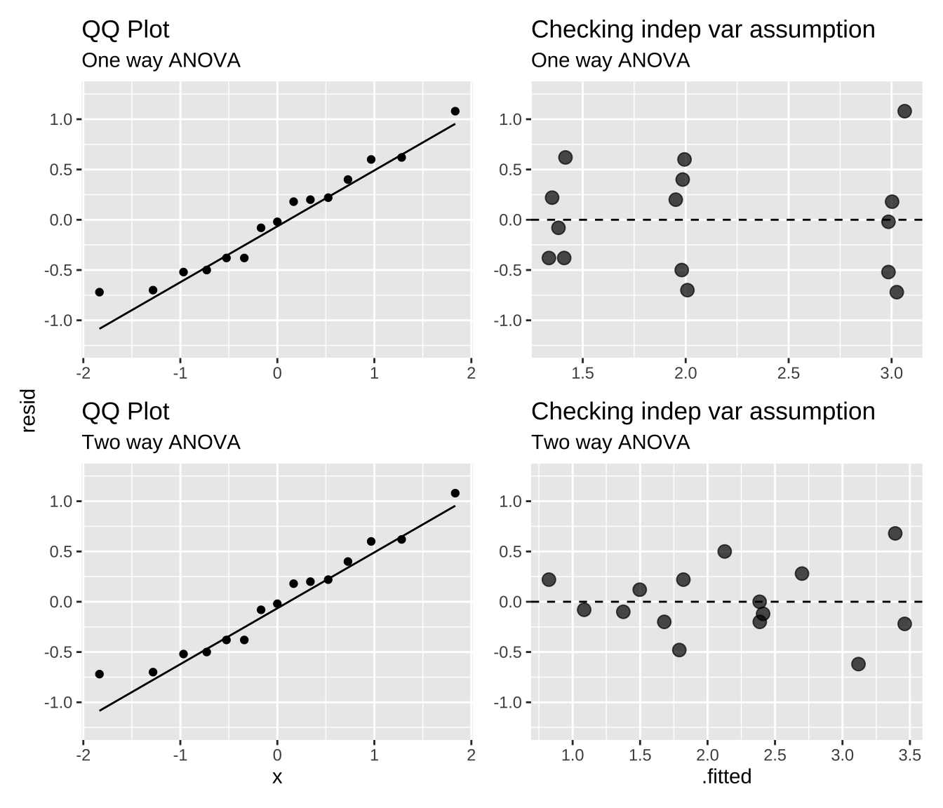
NHST for a randomized block design.
In this model, the null and alternative hypotheses are
- \(H_0:\) There is no association between predator treatment and zooplankton diversity – i.e. Under the null, we predict zooplankton diversity in this experiment as the intercept plus the deviation associated with stream (Figure 2a).
- \(H_A:\) There is an association between predator treatment and zooplankton diversity – i.e. Under the alternative, we predict zooplankton diversity in this experiment as the intercept plus and the deviation associated with stream plus the effect of one or more treatments (Figure 2b).
As in a standard ANOVA, we test the null hypothesis by looking comparing \(F\) for the factor of interest to its null distribution. Partitioning the Sums of Squares for these models is a bit tricky, and requires us to make decisions. We will put this challenge off until late in this section.
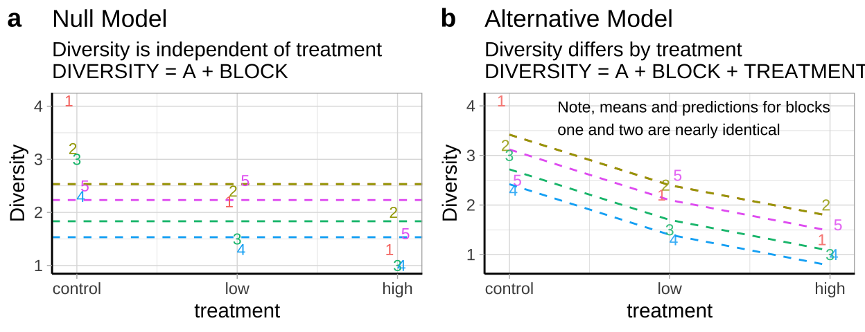
Figure 2: Null (a) and alternative (b) hypotheses for our blocked predation experiment.
NHST for our example:
We can again test the null by running an anova!! We reject the null (\(P_\text{two_way_ANOVA} = 0.0015\)), and conclude that not all treatments are the same. I note that, for this case, we get a similar result if we ignore block, although our p value is a bit higher (\(P_\text{one_way_ANOVA} = 0.0025\)).
anova(zoo_two_way_ANOVA)Analysis of Variance Table
Response: diversity
Df Sum Sq Mean Sq F value Pr(>F)
block 4 2.3400 0.5850 2.7924 0.101031
treatment 2 6.8573 3.4287 16.3660 0.001488 **
Residuals 8 1.6760 0.2095
---
Signif. codes: 0 '***' 0.001 '**' 0.01 '*' 0.05 '.' 0.1 ' ' 1Uncertainty, Post-hoc Tests, and Significance Groups
Note: New package for post-hoc tests – now with significance groups!
I explored the emmeans and multcomp packages and found an easier way to get 95% confidence intervals, conduct post-hoc tests, and identify significance groups. First, we’ll input our model into the emmeans() function, which displays 95% confidence intervals when printed.
library(emmeans)
zoo_two_way_ANOVA_emmeans <- emmeans::emmeans(zoo_two_way_ANOVA, ~ treatment)
zoo_two_way_ANOVA_emmeans
treatment emmean SE df lower.CL upper.CL
control 3.02 0.205 8 2.548 3.49
low 2.00 0.205 8 1.528 2.47
high 1.38 0.205 8 0.908 1.85
Results are averaged over the levels of: block
Confidence level used: 0.95 We can also use this function to conduct a Tukey post-hoc test with the contrast function. Note: Specify method = "pairwise" to obtain Tukey Test results.
emmeans::contrast(zoo_two_way_ANOVA_emmeans,
                  method = "pairwise")  %>%
  tidy()                                                                                                                                                                      %>%  mutate_at(c("estimate", "std.error", "statistic", "adj.p.value"), round, digits = 4) %>%
kbl()| term | contrast | null.value | estimate | std.error | df | statistic | adj.p.value |
|---|---|---|---|---|---|---|---|
| treatment | control - low | 0 | 1.02 | 0.2895 | 8 | 3.5235 | 0.0190 |
| treatment | control - high | 0 | 1.64 | 0.2895 | 8 | 5.6653 | 0.0012 |
| treatment | low - high | 0 | 0.62 | 0.2895 | 8 | 2.1418 | 0.1424 |
Lastly, we can even get significance groups!
| treatment | estimate | std.error | df | conf.low | conf.high | .group |
|---|---|---|---|---|---|---|
| control | 3.02 | 0.2 | 8 | 2.40 | 3.64 | a |
| low | 2.00 | 0.2 | 8 | 1.38 | 2.62 | b |
| high | 1.38 | 0.2 | 8 | 0.76 | 2.00 | b |
Adding significance groups to our plot
We can take this output to add significance groupings to our plot (Figure 3).
ggplot(zoo, aes(x = treatment, y = diversity, color = treatment)) +
  geom_jitter(height = 0, width = .2, size = 4, alpha = .7, show.legend = FALSE) +
  stat_summary(fun.data = mean_cl_normal, geom = "errorbar", width = .2,
               position = position_nudge(x = .4), show.legend = FALSE) +
  geom_text(data = tidy(zoo_sig_groups), aes(label = .group, y = 4.5), size = 8, color = "black") +
  theme(axis.text = element_text(size = 12),
        axis.title = element_text(size = 15))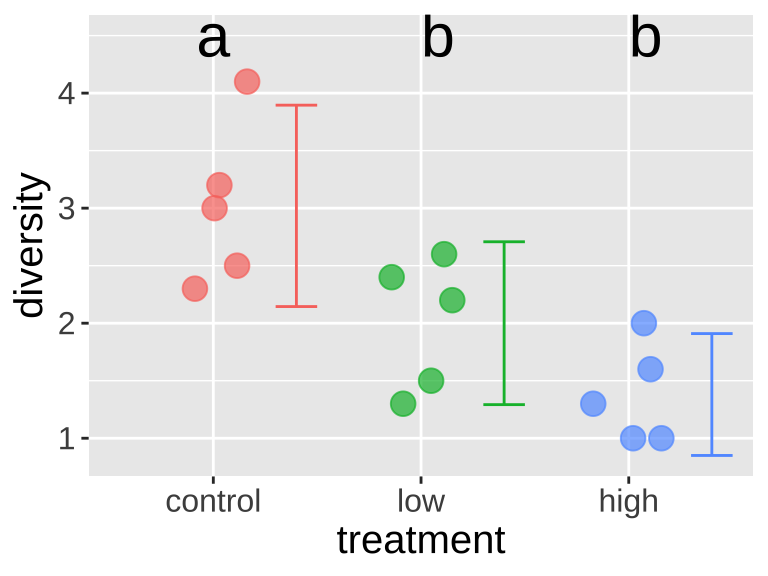
Figure 3: Adding significance groupings to our plot
Comparing 95% CI with one and two way ANOVA
Comparing 95% CI with and without block in our model Including block has decreased uncertainty in our estimates. This will usually happen often to a much greater extent than seen in Figure 4 below – because including block models extraneous variation associated with block.
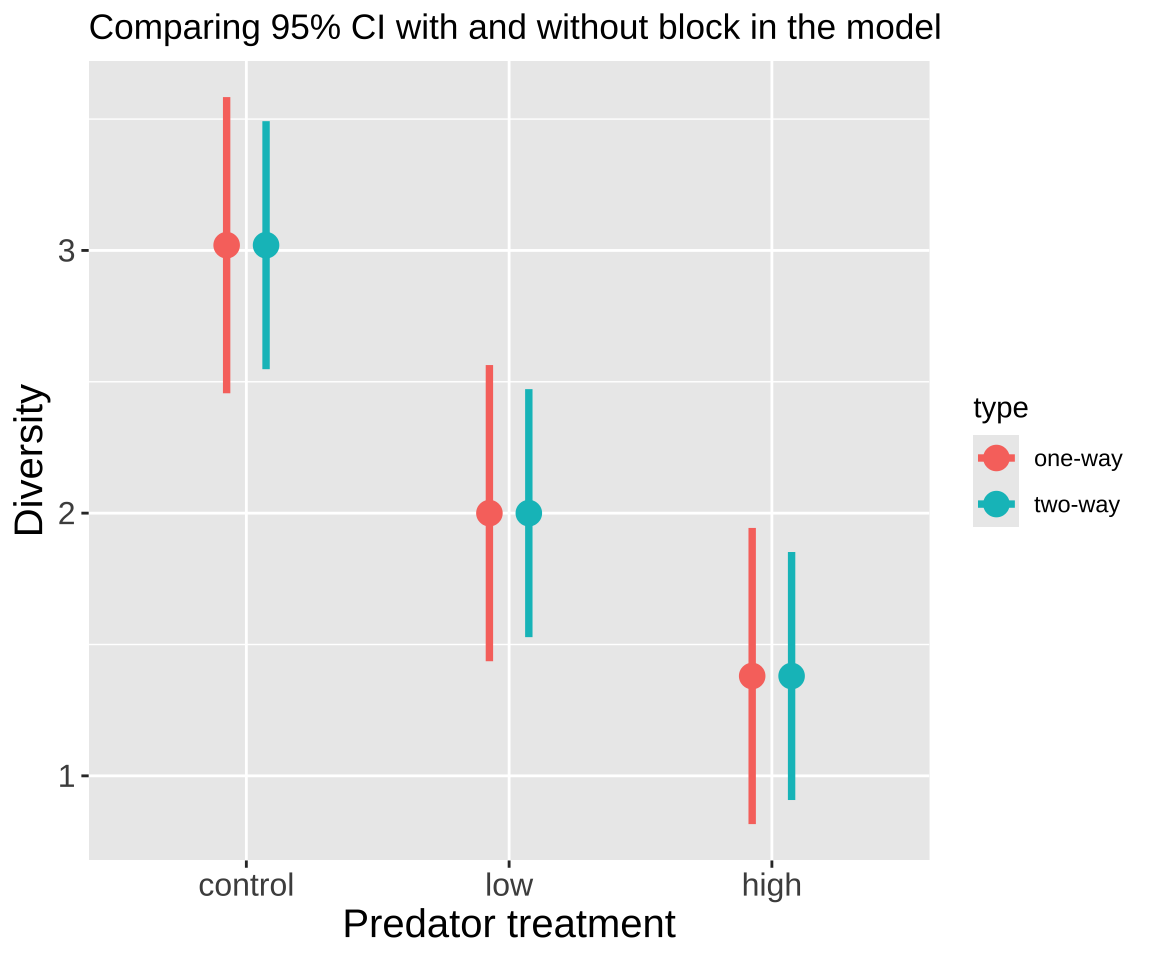
Figure 4: Comparing 95% confidence intervals for the effect of predatory treatment on zooplankton diversity for models with (two-way ANOVA) and without (one-way ANOVA) block included.
Summary
With or without accounting for block, our model performs reasonably well. In both cases, we reject the null and conclude that the presence of fish predators decreases zooplankton diversity. However, in neither case can we detect a significant difference between low and high fish density. That said, we have a lower p-value and tighter confidence intervals when including block in our model.
Types of Sums of Squares
Type I Sums of Squares
Calculating sums of squares sequentially is the default approach in R. Sequential Type I sums of squares calculate the sums of squares for the first term in your model, then the second, the third, and so on. This means that:
- Sums of squares, mean squares, F values, and p-values may change depending on the order in which variables are entered into the model.
- However, parameter estimates and their uncertainty will not change with order.
In general, sequential sums of squares make the most sense when:
- We are not interested in the significance of the earlier terms in our model. These terms may be included to account for variation but are not our main focus.
- Designs are “balanced” (Figure 5), as balanced designs yield the same sums of squares, F, and p-values regardless of the order in which terms are entered into the model.
Unfortunately, Type I sums of squares are usually not the best choice.
.](images/balanced-and-unbalanced-design%20(1).webp)
Figure 5: Examples of balanced and unbalanced statistical designs, from Statistics How To.
Calculating Type I Sums of Squares
To calculate Sequential “Type I” sums of squares we:
- Calculate \(SS_{error}\) and \(SS_{total}\) as we always do! (Figure 6A,D)
- Calculate the \(SS_{thing1}\) (in this case Block), as if it where the only thing in the model, \(\hat{Y}_{i|block}\). (Figure 6B).
- Calculate the \(SS_{thing2}\) (in this case Treatment), as the deviation of predicted values from a model with both things in it, \(\hat{Y}_{i|block,treatment}\), minus predictions from a model with just thing1 in it, \(\hat{Y}_{i|block}\) (Figure 6C).
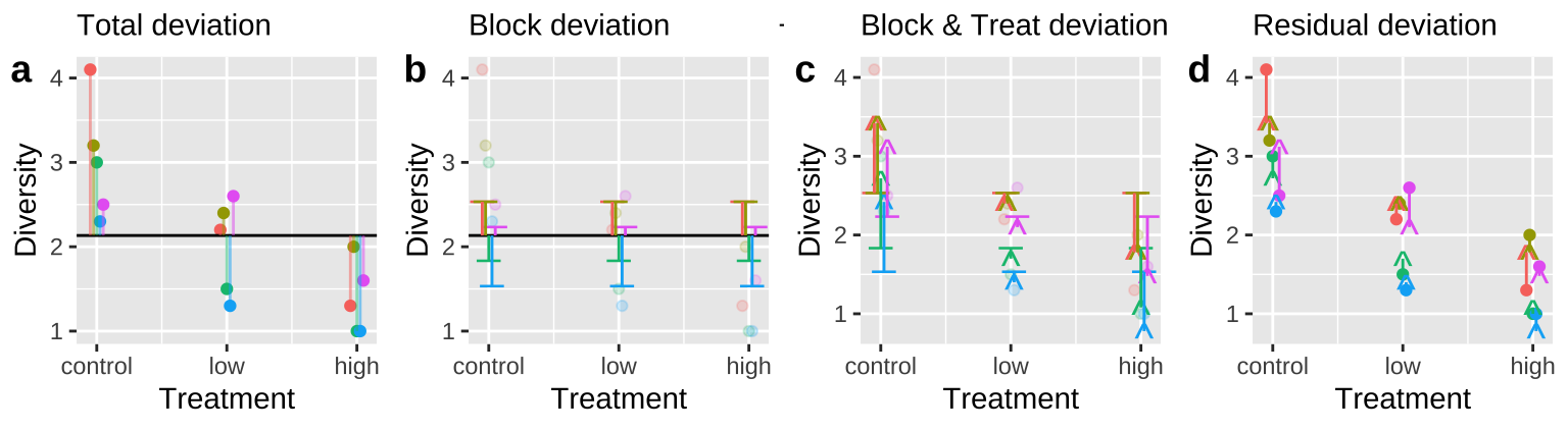
Figure 6: Calculating sequential sums of squares for our zooplankton model. a Total deviations, as usual. b Deviations from predicted values of Block alone without considering the treatment — this makes up \(SS_{block}\). c Deviations of predictions from \(block + treatment\) away from predictions of block alone — this makes up \(SS_{treatment}\). d Deviation of data points from the full model (blue line) — this makes up \(SS_{error}\).
We use the sequential method to calculate sums of squares because we first want to account for “block.” The code below shows how anova() calculates its answer. In our case, we ignore the F-value and significance of block, as it’s included to account for shared variation, not to be tested.
block_model <- lm(diversity ~ block, zoo)
combine_models <- full_join(augment(block_model ) %>%
            dplyr::select(diversity, block, .fitted_block = .fitted,  .resid_block = .resid),
          augment(zoo_two_way_ANOVA) %>%
            dplyr::select(diversity, block, treatment, .fitted_full = .fitted, .resid_full= .resid),
          by = c("diversity", "block"))

combine_models %>%
  summarise(ss_tot    = sum( (diversity      - mean(diversity))^2 ),
            ss_block  = sum( (.fitted_block  - mean(diversity))^2 ),
            ss_treat = sum( (.fitted_full    - .fitted_block)^2 ),
            ss_error  = sum( (diversity      - .fitted_full)^2 ),
            #df
            df_block  = n_distinct(block) - 1,  df_treat = n_distinct(treatment) -1,
            df_error  = n() - 1,
            #
            ms_block  = ss_block  / df_block,
            ms_treat  = ss_treat / df_treat ,
            ms_error  = ss_error  / df_error,
            #
            F_treat   = ms_treat / ms_error,
            p_bmass2   = pf(q = F_treat, df1 = df_treat, df2 = df_error, lower.tail = FALSE))                                                                  %>% mutate_all(round,digits = 4) %>%DT::datatable( options = list( scrollX='400px'))
Compare to:
anova(lm(diversity ~ block + treatment, data = zoo)) %>% tidy() %>% mutate_at(-1,round, digits = 4)%>% kbl()| term | df | sumsq | meansq | statistic | p.value |
|---|---|---|---|---|---|
| block | 4 | 2.3400 | 0.5850 | 2.7924 | 0.1010 |
| treatment | 2 | 6.8573 | 3.4287 | 16.3660 | 0.0015 |
| Residuals | 8 | 1.6760 | 0.2095 | NA | NA |
Type II Sums of Squares:
Since this study is balanced, the order of factors in our model doesn’t affect the results, meaning we get the same answer regardless of factor order. However, in most two-way ANOVAs—particularly with unbalanced designs—the order of factors can impact the results. In these cases, using Type II sums of squares helps us better account for each factor’s unique contribution.
Why Choose Type II Sums of Squares?
When both factors are of interest (not just as controls) and/or the design is unbalanced, Type II sums of squares provide a more interpretable analysis. Type II sums of squares calculate the effect of each factor while controlling for the other, without prioritizing one factor over the other in the sequence, as Type I sums of squares would. This approach prevents misleading conclusions that could arise if factor order impacts the calculated sums of squares.
Steps to Calculate Type II Sums of Squares
To calculate Type II sums of squares, we follow these steps:
Calculate \(SS_{error}\) and \(SS_{total}\) as we normally would for an ANOVA (see Figure 6A, D).
Compute sums of squares for individual factors by fitting models with each factor alone:
- \(\text{SS}_\text{model -- block only}\), which captures the variability explained by block alone.
- \(\text{SS}_\text{model -- treatment only}\), which captures the variability explained by treatment alone.
Compute sums of squares for the full model that includes both factors, \(\text{SS}_\text{model -- block & treatment}\). This step helps us understand the combined explanatory power of both factors.
Calculate sums of squares for each factor as if it were the second term in a Type I model, meaning each factor’s effect is measured after accounting for the other factor’s effect. Specifically:
- \(\text{SS}_\text{block}\) is obtained by comparing predicted values from the full model (block and treatment) \(\hat{Y}_{i|block,treatment}\) to predictions from the model with only treatment, \(\hat{Y}_{i|treatment}\). This captures block’s effect after accounting for treatment.
- \(\text{SS}_\text{treatment}\) is calculated by comparing predicted values from the full model \(\hat{Y}_{i|block,treatment}\) to predictions from the model with only block, \(\hat{Y}_{i|block}\). This isolates the effect of treatment after accounting for block.
We can use the Anova() function in the car package to specify what types of Sums Of Squares You want to calculate. As discussed previously - this is a case hwere it really doesn’t matter. As you can see
library(car)
Anova(lm(diversity ~  treatment + block, data = zoo), type = "II")                                                                                                              %>% tidy() %>% mutate_at(-1,round, digits = 4)
# A tibble: 3 × 5
term sumsq df statistic p.value
<chr> <dbl> <dbl> <dbl> <dbl>
1 treatment 6.86 2 16.4 0.0015
2 block 2.34 4 2.79 0.101
3 Residuals 1.68 8 NA NA When to Use Type II vs. Type I Sums of Squares
If the design is balanced, Type I sums of squares often yield the same results as Type II, since each factor’s contribution to the model is equal regardless of order. However, in unbalanced designs, using Type I sums of squares can give misleading results because it calculates Sums Of Squares sequentially in the order entered into R. This means that the p-value for the frst thing in the model will be calculated without accounting for the second thing, when using type I Sums of Squares, but this issue goes away with type II sums of square. As such, Type II sums of squares are more appropriate when factor order should not dictate importance or when we want to interpret each factor’s effect independently of the other.
Two way ANOVAs with interaction.
Statistical interactions
Above, we assumed the treatment effect was consistent across all blocks (or groups) — i.e., the impact of the treatment was the same regardless of the specific block. However, we often encounter cases where the effect of a treatment might differ depending on the context or specific characteristics of each block. This variation in treatment effects across blocks is what we refer to as an “interaction effect.”
Consider the example of patients taking two different medications. Suppose each medication has its own set of side effects. When a patient is prescribed both medications simultaneously, we might be concerned that the combination could produce side effects that are not just a simple addition of the side effects of each medication individually. Instead, there could be an interaction effect, where the combination of both medicines leads to a more severe or unexpected outcome. This means the effect of one medicine depends on whether the patient is also taking the other medicine, creating a unique outcome that wouldn’t be predicted by simply adding up the effects of each medicine independently (read a review of drug interactions here). This is why your physician or pharmacist often asks what other drugs your taking.
I like orange juice in the morning. I also like the taste of minty fresh toothpaste. But drinking orange juice after brushing my teeth tastes terrible.
This is an example of an interaction.
- On its own, toothpaste tastes good.
- On its own OJ is even better.
- Put them together, and you have something gross.
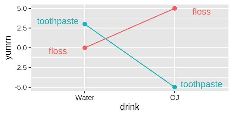
This is an extreme case. More broadly, an interaction is any case in which the slope of two lines differ – that is to say when the effect of one variable on an outcome depends on the value of another variable.
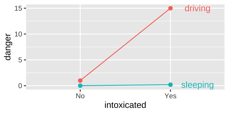
Another example of an interaction Getting intoxicated is a bit dangerous. Driving is a bit dangerous. Driving while intoxicated is more dangerous than adding these up individually.
Visualizing main & interactive effects
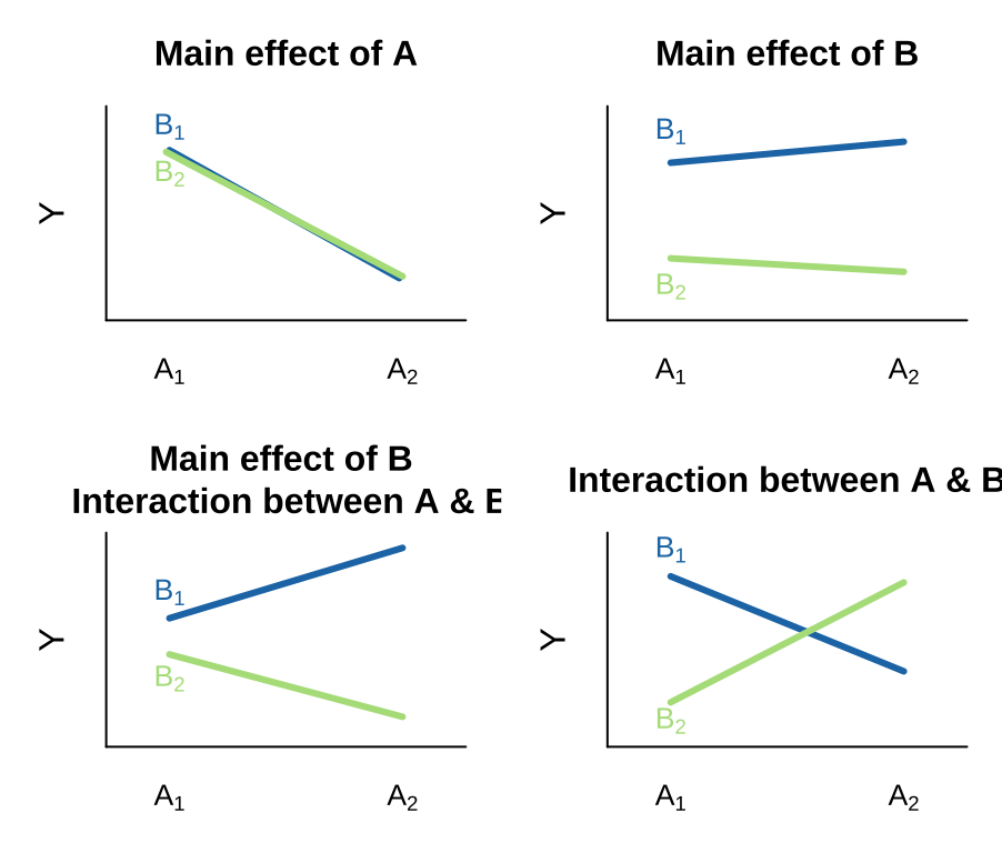
There are many possible outcomes when looking into a model with two predictors and the potential for an interaction. I outline a few extreme possibilities, plotted on the right.
- We can see an effect of only variable A on Y. That is, lines can have nonzero slopes (“Main effect of A”).
- We can see a effect of only variable B on Y. That is, lines can have zero slopes but differing intercepts (“Main effect of B”).
- We can see an effect of only variable B on Y, but an interaction between that variable and the other. That is, intercepts and slopes can differ (or vice versa) in such a way that the mean of Y only differs by one of the explanatory variables (e.g. “Main effect of B, Interaction between A & B”). and/or
- We can have only an interaction. That is, on their own values of A or B have no predictive power, but together they do. (different slopes)
Interaction Case Study
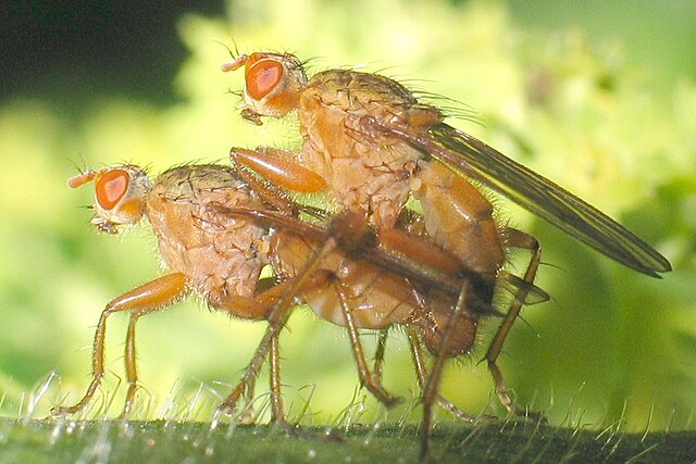
Females of the yellow dung fly, Scathophaga stercoraria, mate with multiple males, leading to “sperm competition” among different males to fertilize her eggs.
What determines a sperm’s competitiveness? To explore this, Hosken, Blanckenhorn, and Garner (2002) tested whether the origin of males and females (from the UK or Switzerland) and their interaction influenced the percentage of offspring sired by the second male.
Our model is:
\[\text{SIRING }2^\text{ND} \text{MALE} = \text{FEMALE }+\text{ MALE }+\text{ FEMALE } \times \text{MALE}\]
Biological Hypotheses
There are a few possibilities:
- Females from the UK populations may reject (or accept) more sperm from the second male than females from Switzerland (main effect of female population).
- Sperm from UK males may have higher (or lower) siring success than sperm from Swiss males (main effect of male population).
- Alternatively, sperm from Swiss males might have high siring success with Swiss females, while UK male sperm has high success with UK females, suggesting harmonious co-adaptation (interaction).
- Or perhaps females have evolved to resist local sperm, so sperm from Swiss males has high success with UK females but low success with Swiss females, suggesting intersexual conflict.
The Data
The raw data are available here if you’d like to follow along. Note that I modified the dataset slightly for teaching purposes by changing the first data point to reflect a mating between a UK female and a Swiss male.
dung_link <- "https://raw.githubusercontent.com/ybrandvain/datasets/refs/heads/master/dung.csv"
dung <- read_csv(dung_link)
From the means and standard errors below, we observe:
- UK males have similar mating success with both UK and Swiss females.
- Swiss males appear to have notably lower success with Swiss females but higher success with UK females, suggesting a history of intersexual conflict over the success of the second male.
| female | swiss male | uk male |
|---|---|---|
| swiss | 59.73 (2.6) | 73.14 (1.9) |
| uk | 92.6 (1.7) | 71.81 (2.6) |
Fitting a Linear Model with an Interaction in R
In R, we can specify an interaction term along with main effects using a colon, :, or specify a full model with *. Thus, the two models below are identical:
lm_dung_fmi <- lm(sire.2nd.male ~ female + male + female:male, dung)
lm_dung_fmi <- lm(sire.2nd.male ~ female * male, dung)
broom::tidy(lm_dung_fmi)
# A tibble: 4 × 5
term estimate std.error statistic p.value
<chr> <dbl> <dbl> <dbl> <dbl>
1 (Intercept) 59.7 2.30 26.0 6.21e-33
2 femaleuk 32.9 3.25 10.1 3.05e-14
3 maleuk 13.4 3.31 4.05 1.57e- 4
4 femaleuk:maleuk -34.2 4.60 -7.43 6.70e-10As usual, we can examine our estimates and uncertainties using summary.lm() or equivalently, the tidy() function. As with most linear models, note that these p-values and t-values (shown as statistic in tidy()) may not necessarily reflect the biological questions we care about and can sometimes be misleading.
Still, we can use this output to make predictions. The first terms should look familiar. For the final term, femaleuk:maleuk, we multiply femaleuk (0 or 1) by maleuk (0 or 1). This interaction term is 1 only when both the male and female are from the UK, resulting in a 34.2% reduction in siring success compared to the additive effect of male UK and female UK. Because femaleuk (0 or 1) multiplied by maleuk (0 or 1) is zero in all other cases, this effect only applies to this specific cross.
We can see this pattern in the design matrix below. Remember, for those interested in linear algebra, we make predictions as the dot product of our model coefficients and the design matrix.
model.matrix(lm_dung_fmi) %>%data.frame() %>% tibble()# A tibble: 60 × 4
X.Intercept. femaleuk maleuk femaleuk.maleuk
<dbl> <dbl> <dbl> <dbl>
1 1 1 1 1
2 1 0 1 0
3 1 0 1 0
4 1 0 1 0
5 1 0 1 0
6 1 0 1 0
7 1 0 1 0
8 1 0 1 0
9 1 0 1 0
10 1 0 1 0
# ℹ 50 more rowsIf you prefer not to work with linear algebra, the model predicts second male siring success as follows:
\[ \begin{array}{cccccc} & \text{Intercept} &\text{Female UK?}&\text{Male UK?}&\text{Both UK?}&\widehat{Y_i}\\ \widehat{Y}_\text{female.swiss x male.swiss} = &59.733 \times 1+ &32.867 \times 0 + &13.410 \times 0 -&34.197\times 0 =&59.733\\ \widehat{Y}_\text{female.swiss x male.uk} = &59.733 \times 1+ &32.867 \times 0 + &13.410 \times 1 -&34.197\times 0 =&73.14\\ \widehat{Y}_\text{female.uk x male.swiss} = &59.733 \times 1+ &32.867 \times 1 + &13.410 \times 0 -&34.197\times 0 = &92.60\\ \widehat{Y}_\text{female.uk x male.uk} = &59.733 \times 1+ &32.867 \times 1 + &13.410 \times 1 -&34.197\times 1 = &71.83\\ \end{array} \]
We can see that the model predictions simply describe our four sample means.
Hypothesis testing
Statistical hypotheses
We can translate the biological hypotheses into three pairs of statistical null and alternative hypotheses.
We examine three null and alternative hypotheses
- Main effect of Male
- \(H_0:\) Siring success is independent of male origin.
- \(H_A:\) Siring success differs by male origin.
- \(H_0:\) Siring success is independent of male origin.
- Main effect of Female
- \(H_0:\) Siring success is independent of female origin.
- \(H_A:\) Siring success differs by female origin.
- \(H_0:\) Siring success is independent of female origin.
- Interaction between Male and Female
- \(H_0:\) The influence of male origin on siring success does not differ by female origin.
- \(H_0:\) The influence of male origin on siring success is depends on female origin.
- \(H_0:\) The influence of male origin on siring success does not differ by female origin.
We visualize these hypotheses below
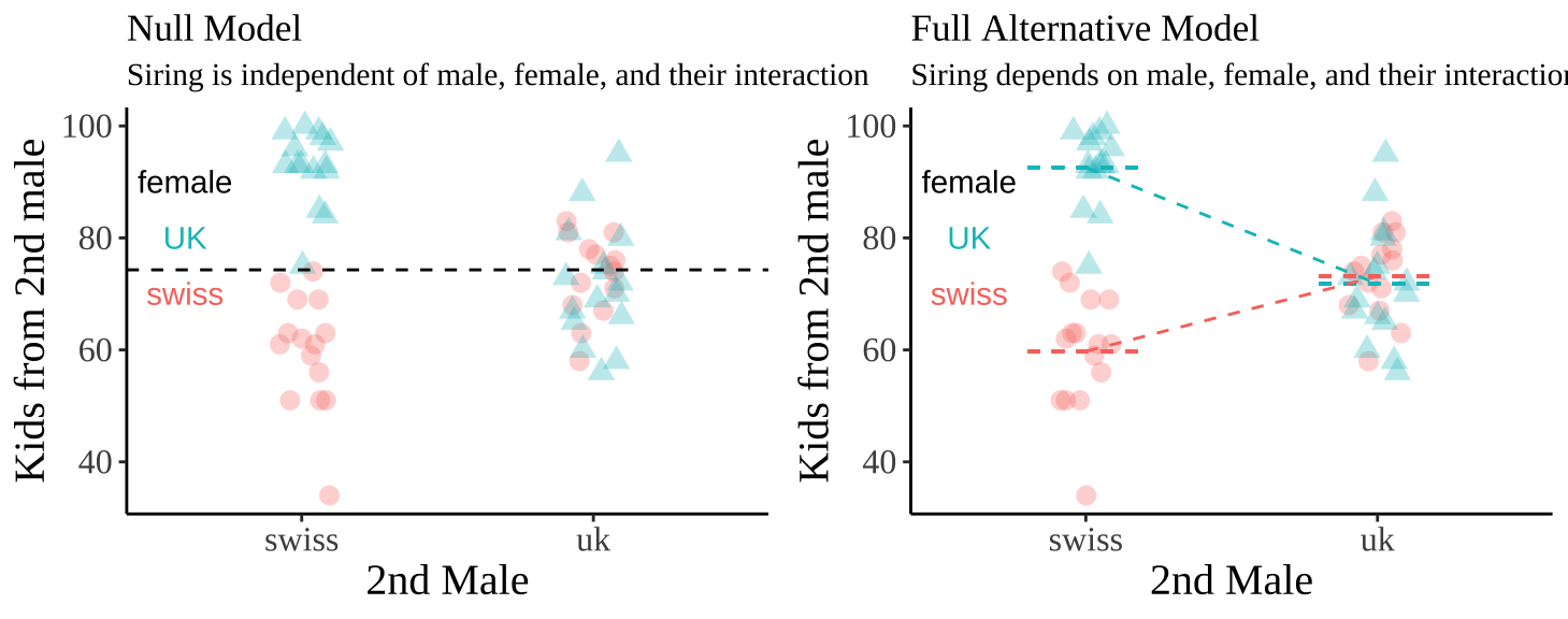
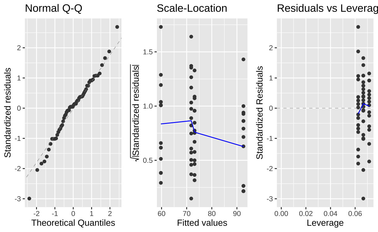
Evaluating Assumptions
Linear models rely on the following assumptions:
- Linearity: Observations can be adequately modeled by adding up predictions in the model equation.
- Homoscedasticity: The variance of residuals is constant across all predicted values (\(\hat{Y_i}\)) and is consistent for any value of X.
- Independence: Observations are independent of one another (except as explained by predictors in the model).
- Normality: Residual values are normally distributed.
- Data Collection Without Bias: As always, ensure data is unbiased.
Examining our diagnostic plots, the data appears to meet these assumptions. We visualize this using the autoplot() function from the ggfortify package:
Hypothesis Testing in an ANOVA Framework: Types of Sums of Squares
tl/dr
- In more complex linear models, we need fair methods to attribute variance:
- Type I Sums of Squares (via
anova()function) are useful when we want to account for a “covariate.” The order of terms affects p-values and F-values with Type I Sums of Squares.
- Type II Sums of Squares work well when we are equally interested in each main effect as a hypothesis.
- Type III Sums of Squares are appropriate when both main effects and interactions are of interest.
- Type I Sums of Squares (via
We can specify the type of sums of squares using the Anova() function from the car package. When data is balanced, Type I and Type II sums yield the same results. However, these methods can behave differently with unbalanced designs.
In our case, Type III Sums of Squares are likely the best choice.
Type I Sums of Squares
In the previous chapter, we used Type I sums of squares, where variable order matters. Typically, we first add variables we’re less interested in but might confound results.
- Sums of Squares for the First Variable, \(SS_A\):
- Fit a model with only the first variable (A) and calculate the sums of squares for the difference between predictions from this model and the grand mean.
- Sums of Squares for the Second Variable, \(SS_B\):
- Fit a model with both variables (A and B) and calculate the difference between predictions from this model and the previous, assigning the result to \(SS_B\).
- Interaction Term, \(SS_{A:B}\):
- Fit a model with all main effects and the first interaction (e.g.,
A:B) and calculate the sums of squares as the difference between predictions with and without the interaction term.
- Fit a model with all main effects and the first interaction (e.g.,
To compute Type I sums of squares:
anova(lm_dung_fmi)Analysis of Variance Table
Response: sire.2nd.male
Df Sum Sq Mean Sq F value Pr(>F)
female 1 3676.4 3676.4 46.4031 7.074e-09 ***
male 1 271.9 271.9 3.4324 0.0692 .
female:male 1 4375.6 4375.6 55.2292 6.695e-10 ***
Residuals 56 4436.7 79.2
---
Signif. codes: 0 '***' 0.001 '**' 0.01 '*' 0.05 '.' 0.1 ' ' 1Type I sums can be misleading if we’re equally interested in both variables, as results may vary with variable order. Compare anova(lm_dung_fmi) with anova(lm_dung_mfi):
Analysis of Variance Table

Response: sire.2nd.male
            Df Sum Sq Mean Sq F value    Pr(>F)
male         1  209.1   209.1  2.6388    0.1099
female       1 3739.2  3739.2 47.1967 5.674e-09 ***
male:female  1 4375.6  4375.6 55.2292 6.695e-10 ***
Residuals   56 4436.7    79.2
---
Signif. codes:  0 '***' 0.001 '**' 0.01 '*' 0.05 '.' 0.1 ' ' 1
In this case, the results are similar, but that isn’t always true.
Type II Sums of Squares
When both variables are of interest, we use “Type II Sums of Squares,” which are independent of variable order.
- Sums of Squares for Each Main Effect, \(SS_X\):
- Fit a model with all main effects except X (model
no_x). - Fit a full model with all main effects (model
main). - Calculate \(SS_X\) as the squared difference between predictions from these two models.
- Fit a model with all main effects except X (model
For interactions, follow a similar approach.
To calculate Type II sums of squares:
Anova Table (Type II tests)

Response: sire.2nd.male
            Sum Sq Df F value    Pr(>F)
female      3739.2  1 47.1967 5.674e-09 ***
male         271.9  1  3.4324    0.0692 .
female:male 4375.6  1 55.2292 6.695e-10 ***
Residuals   4436.7 56
---
Signif. codes: 0 '***' 0.001 '**' 0.01 '*' 0.05 '.' 0.1 ' ' 1Anova(lm_dung_mfi, type = "II")Anova Table (Type II tests)
Response: sire.2nd.male
Sum Sq Df F value Pr(>F)
male 271.9 1 3.4324 0.0692 .
female 3739.2 1 47.1967 5.674e-09 ***
male:female 4375.6 1 55.2292 6.695e-10 ***
Residuals 4436.7 56
---
Signif. codes: 0 '***' 0.001 '**' 0.01 '*' 0.05 '.' 0.1 ' ' 1Type II Sums of Squares have unique characteristics:
- They don’t sum to the total sums of squares.
- Main effects are considered without their interactions, which can be conceptually odd.
Type III Sums of Squares
When interested in both main effects and interactions, Type III Sums of Squares compares the full model predictions with those excluding the variable or interaction of interest. Variable order is irrelevant, and interacrions are not held out for last.
Anova(lm_dung_fmi, type = "III")Anova Table (Type III tests)
Response: sire.2nd.male
Sum Sq Df F value Pr(>F)
(Intercept) 53521 1 675.545 < 2.2e-16 ***
female 8102 1 102.259 3.046e-14 ***
male 1302 1 16.435 0.000157 ***
female:male 4376 1 55.229 6.695e-10 ***
Residuals 4437 56
---
Signif. codes: 0 '***' 0.001 '**' 0.01 '*' 0.05 '.' 0.1 ' ' 1Biological Conclusions for Case Study
We conclude that female (F = 102.259, df = 1, p = \(3 \times 10^{-14}\)), male (F = 16.4, df = 1, p = 0.00016), and their interaction (F = 55.2, df = 1, p = \(6.7 \times 10^{-10}\)) all impact the siring success of the second male. Notably, when both females and second males are from the UK, siring success is significantly lower than expected based on each main effect alone. This suggests that sexual conflict in the UK may influence second sperm competitiveness. Future studies could explore why the siring success of second males from Sweden remains unaffected by the maternal population origin.
Quiz
Figure 7: Quiz on the two way ANOVA here
Functions and packages introduced
Diagnostic and Visualization Functions
autoplot() (from the ggfortify package): Provides a quick way to visualize diagnostic plots for linear models. This function simplifies residual analysis by generating diagnostic plots with one command.
Post-Hoc Analysis and Contrasts
emmeans() (from the emmeans package): Computes estimated marginal means for factors in the model. It is useful for exploring main and interaction effects in a Two-Way ANOVA, especially in post-hoc comparisons.
contrast() (from the emmeans package): Allows for custom contrasts between estimated marginal means, making it easier to examine specific hypotheses about factor level differences.
Compact Letter Display
cld() (from the multcomp package): Generates a compact letter display for post-hoc test results, which helps visualize groups that are not significantly different from each other.
ANOVA with Type II and Type III Sums of Squares
Anova() (from the car package): Provides flexible options for calculating Type II and Type III sums of squares in ANOVA models, which are especially useful in models with interaction terms.