Motivating scenarios:
You want to understand the intellectual foundation for a fundamental challenge in statistics.
Learning goals: By the end of this chapter, you should be able to:
- Differentiate between a parameter and an estimate.
- Describe the different ways sampling can go wrong (sampling bias, non-independence, and sampling error) that make estimates deviate from parameters, and how to recognize and mitigate these issues.
- Describe the sampling distribution and why it is useful.
- Use
Rto build a sampling distribution from population data.
- Explain the standard error.
- Understand how sample size influences sample estimates.
Populations Have Parameters
The palmerpenguins dataset we’ve been looking at consists of 344 penguins from three species. In this sample, there are 152 Adelie penguins, 68 Chinstrap penguins, and 124 Gentoo penguins. For now, let’s pretend this is a census—i.e., let us assume this represents all penguins on these three islands. In this census, we see that \(\frac{68}{344} = 19.8\%\) of the population are Chinstrap penguins.
In a real sense, the calculation above is a population parameter—it is the true value of the proportion of Chinstrap penguins in this dataset (though it is not a parameter for the entire world population of penguins, it is for this example).
In frequentist statistics, population parameters are the TRUTH—they represent the world as it truly is, either from a population census or from some process that generates data with specific characteristics (e.g., flipping a coin, recombining chromosomes, responding to a drug, etc.). In our example, the entire census data is presented in the table below (Figure 1).
Figure 1: The entire population of our penguins dataset (presented in random order).
Estimate population parameters by sampling
It is usually too much work, costs too much money, or takes too much time to characterize an entire population and calculate its parameters.
So, we take estimates from a sample of the population. This is relatively easy to do in R if we already have a population. We can use the slice_sample() function, with the arguments being the tibble of interest and n as the size of our sample. The sample of 30 penguins in the table below contains 3 Chinstrap penguins. So, 10% of this sample are Chinstrap penguins—a difference of about 9.77% from the true population parameter of 19.8%. Figure 3 compares the census proportion of each species (i.e., the data we have, shown in lighter colors) to a random sample of thirty penguins from our data (in darker colors).
penguins_sample <- slice_sample(penguins, n = 30, replace = FALSE) Figure 2: A sample of size 30 from our larger penguins dataset.
bind_rows(dplyr::mutate(penguins, data = "population (true parameter)"),
          dplyr::mutate(penguins_sample, data = "sample (parameter estimate)")) %>%
  group_by(data, species) %>%
  tally()%>%
  mutate(propotion = n/sum(n)) %>%
  ggplot(aes(y = data, x = propotion, fill = species, alpha= data))+
  geom_col(show.legend = FALSE)+
  facet_wrap(~species,ncol=1)+
  theme(strip.text = element_text(size = 15),axis.text = element_text(size = 15),axis.title = element_text(size = 15))+
  scale_alpha_manual(values = c(.3,1))+
  scale_x_continuous(limits = c(0,1), breaks = c(0,.5,1), labels = c("0","1/2","1"))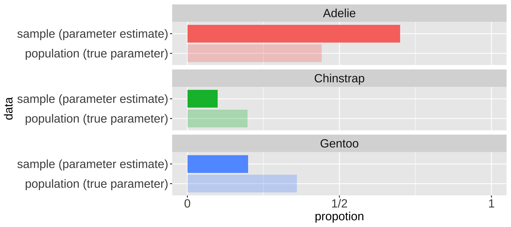
Figure 3: Comparing the proportion of each species in the sample of size 30 (i.e.e the sample estimate) to its actual parameter value in the census (i.e. the true proportion, light colors)
Review of Sampling
Of course, if we already had a well-characterized population, there would be no need to sample—we would just know the actual parameters, and there would be no need to do statistics. But this is rarely feasible or practical, and we’re therefore left with taking samples and doing statistics.
As such, being able to imagine the process of sampling—how we sample and what can go wrong in sampling—is perhaps the most important part of being good at statistics. I recommend walking around and imagining sampling in your free time.
(Avoiding) Sampling Bias
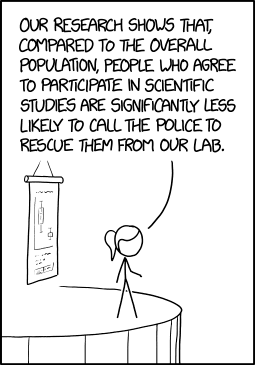
Figure 4: Example of sampling bias from xkcd. Accompanying text: fMRI testing showed that subjects who dont agree to participate are much more likely to escape from the machine mid-scan.
Say we were interested in knowing whether Chinstrap penguins in our dataset have shorter or longer bills than the other penguin species. We could take our 30 individuals from the randomly generated sample above and estimate bill lengths for all three species. If all species’ estimates are unbiased, and individuals are sampled independently, we only have to deal with sampling error, which is discussed below. But if we cannot randomly collect penguins, then we have to deal with bias and non-independence in our sampling.
But it’s often even worse—we don’t have a list of possible subjects to pick from at random. So, what do we do? Say we want a good poll for the presidential election to predict the outcome. Should we build an online survey? Try calling people? Go to the campus cafeteria? Each of these methods could introduce some deviation between the true population parameters and the sample estimate. This deviation is called sampling bias, and it can undermine all the statistical techniques we use to account for sampling error. This is why polling can be so difficult.
Let’s think about this in terms of our dataset. To be more specific, our dataset covers three islands. If we only sampled from Dream Island, we would estimate that 68 of 124 penguins (i.e., 55%) are Chinstrap penguins.
penguins %>%
  dplyr::filter(island == "Dream",.preserve = )%>%
  group_by(species) %>%
  tally()%>%
  complete(species, fill = list(n = 0))
# A tibble: 3 × 2
species n
<fct> <int>
1 Adelie 56
2 Chinstrap 68
3 Gentoo 0When designing a study, do everything you can to eliminate sampling bias. When conducting your own analysis or evaluating someone else’s, always consider how sampling bias could lead to misleading conclusions.

(Avoiding) Non-Independence of Samples
One last important consideration of sampling is the independence of samples.
- Samples are independent if sampling one individual does not change the probability of sampling another.
- Samples are dependent (also called non-independent) if sampling one individual changes the probability of sampling another.
Say we want to estimate the proportion of penguins that are Chinstrap. If we visit an (imaginary) island where all species are, on average, equally likely to be found, but individuals of each species tend to cluster together, we might find a spot with some penguins and start counting. In this case, our sample would be dependent—once we find one penguin, others nearby are more likely to be of the same species than they would be if we randomly selected another location to sample.
Near the end of the term, we will explore ways to account for non-independence. For now, understand that dependence alters the sampling process and requires us to use more complex models.
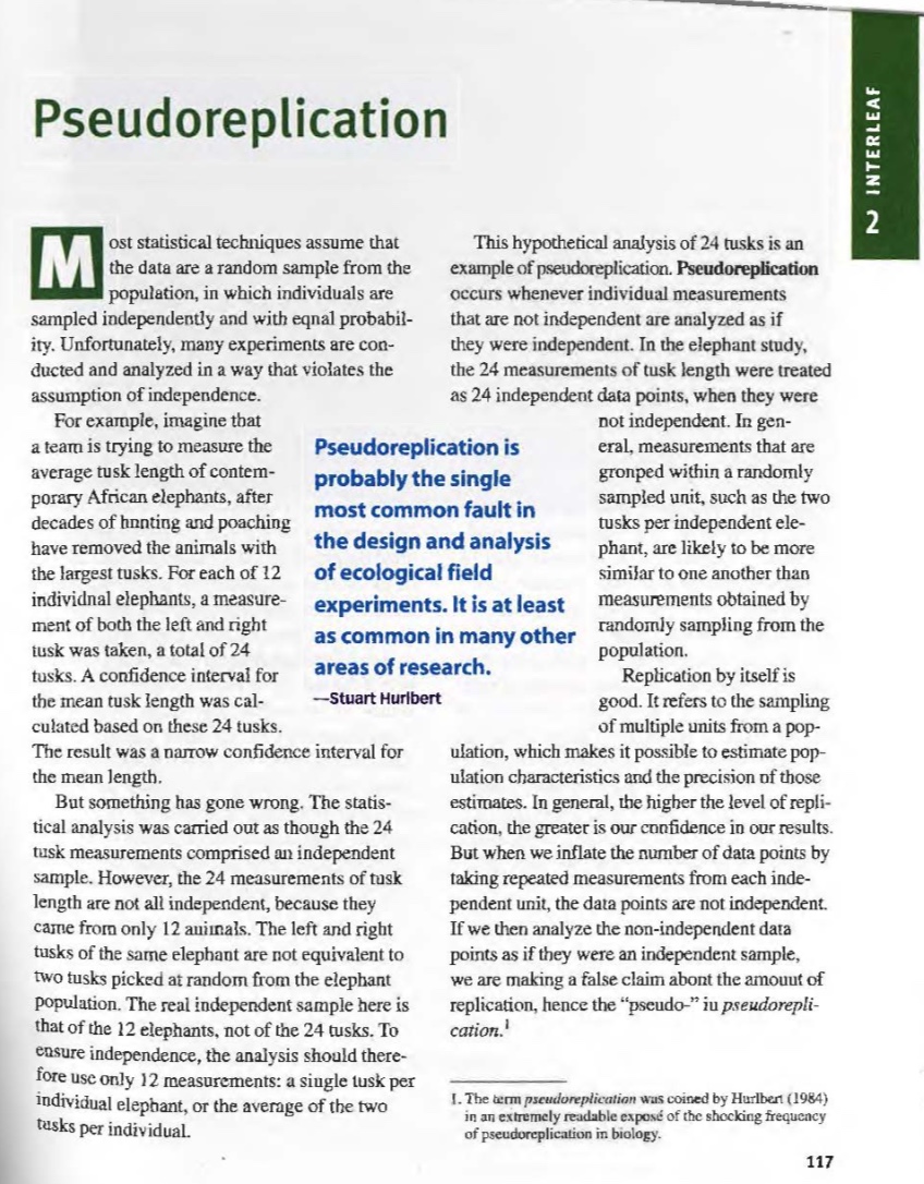
When designing an experiment, or evaluating someone else’s, we should be concerned about pseudo-replication— the term used for non-independent replication (See Fig. 5).
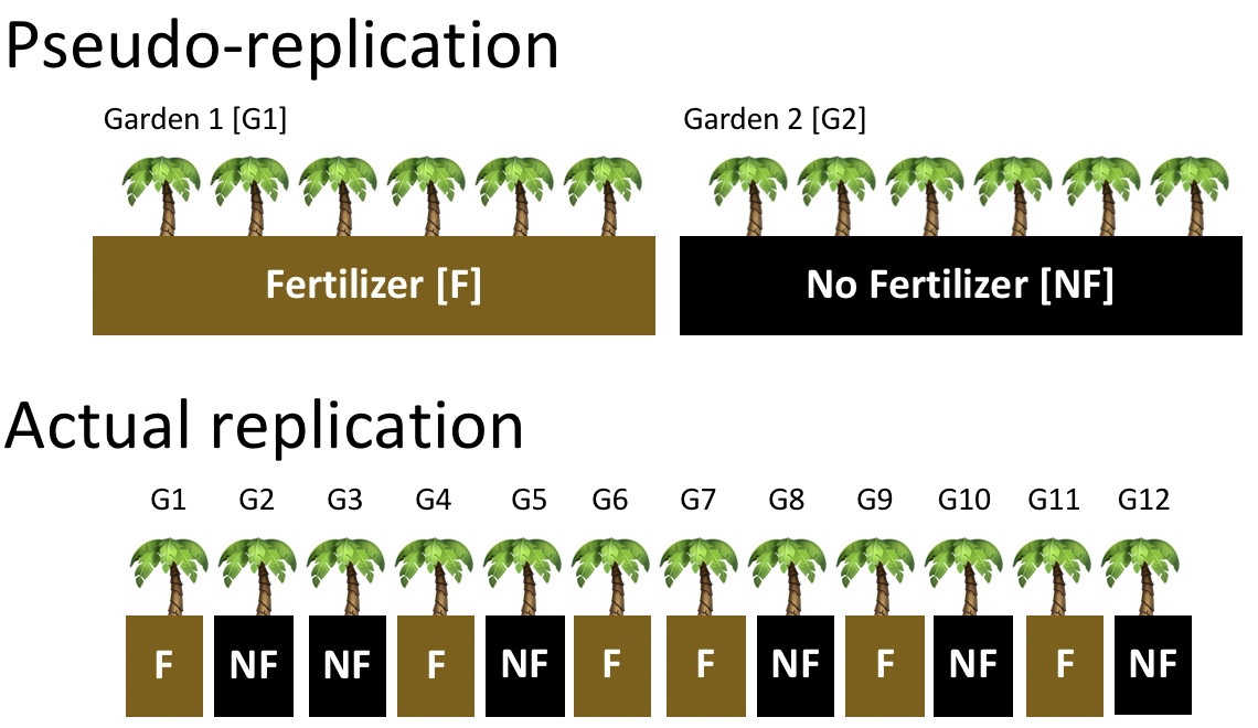
Figure 5: Comparing pseudo-replication (top) to independent replication (bottom). With pseudo-replication the effect of our experimental intervention (in this case fertilizer), is tied up with differences between environments unrelated to treatment (in this case, differences between gardens). Separating treatment and garden, and randomly placing treatments onto garden removes this issue.
There Is No Avoiding Sampling Error
Estimates from samples will differ from population parameters due to chance. This is called sampling error (introduced previously). But make no mistake — sampling error cannot be avoided. We’ve just seen an example of sampling error when our estimate of the proportion of faculty at the College of the Atlantic deviated from the true parameter.
Larger samples and more precise measurements can reduce sampling error, but it will always exist because we take our samples by chance. In fact, I would call it the rule of sampling rather than sampling error.
Much of the material in this chapter — and about half of the content for the rest of this term — focuses on how to handle the law of sampling error. Sampling error is the focus of many statistical methods.
The Sampling Distribution
Let’s say you’ve collected data for a very well-designed study, and you’re excited about it (as you should be!). 🎉 CONGRATS!🎉 Stand in awe of yourself and your data — data is awesome, and it’s how we understand the world.
But now consider this: We know that the law of sampling error means that estimates from our data will differ from the true values due to chance. So, you start to wonder, “What other outcomes might have occurred if things had gone slightly differently?”
The sampling distribution is our tool for exploring the alternate realities that could have been. The sampling distribution is a histogram of the estimates we would get if we repeatedly took random samples of size \(n\). By considering the sampling distribution, we recognize the potential spread of our estimate.
I keep emphasizing how important sampling and the sampling distribution are. So, when, why, and how do we use them in statistics? There are two main ways:
First, when we make an estimate from a sample, we build a sampling distribution around this estimate to describe the uncertainty in our estimate (see the upcoming section on Uncertainty).
Second, in null hypothesis significance testing (see the upcoming section on Hypothesis Testing), we compare our statistics to their sampling distribution under the null hypothesis to assess how likely the results were due to sampling error.
Grasping the concept of the sampling distribution is critical to understanding our goals this term. It requires imagination and creativity because we almost never have or can create an actual sampling distribution (since we don’t have access to the full population). Instead, we have to imagine what it would look like under some model given our single sample. That is, we recognize that we only have one sample and will not take another, but we can imagine what estimates from another round of sampling might look like. Watch the first five minutes of the video below for the best explanation of the sampling distribution I’ve come across.
Figure 6: Watch the first 5 minutes of this explanation of the sampling distribution. Burn this into your brain.
Building a Sampling Distribution
Imagining a sampling distribution is very useful, but we need something more concrete than our imagination. So, how do we actually generate a useful sampling distribution?
Building a Sampling Distribution by Repeatedly Sampling
The most conceptually straightforward way to generate a sampling distribution is to take a bunch of random samples from our population of interest. Below, I repeated the code several times so you can get a sense of what we are doing.
However, saving and recording each sample manually is tedious, so I’ll show you how to have R do this for us below.
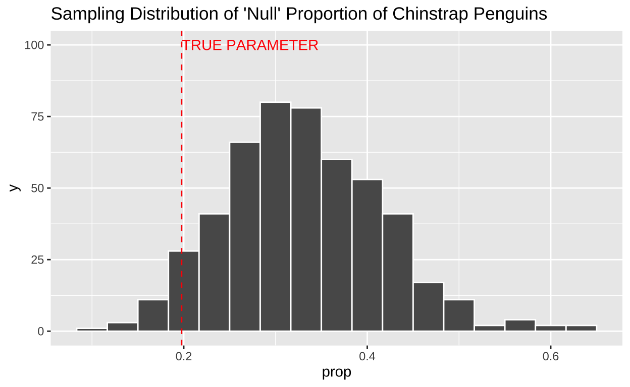
Figure 7: Shows the different estimates of the proportion of Chinstrap penguins with an unbiased and independent sample of size 30 — building a histogram of sample estimates if we were to sample many times. This histogram is known as the sampling distribution.
We can create a sampling distribution by resampling from a population, replicating our code multiple times using the replicate() function. For formatting reasons, we need to set the argument simplify = TRUE inside replicate() and then pipe this output into the bind_rows() function. The code below shows how we can generate the data for Figure 7.
Building a Sampling Distribution
While this approach is conceptually straightforward, it’s also impractical in practice — there’s no reason to characterize an entire population and then resample from it to make an estimate. More often, we have an estimate from a single sample and need a way to consider the sampling distribution.
Building a Sampling Distribution by Simulation
If we have some sense (or hypothesis) of how our population might behave, we can simulate data from it. Like most programming languages, R allows for incredibly complex simulations (I’ve simulated whole genomes), but for now, let’s simulate the process of sampling using the sample() function.
For example, we can generate a sample from a population where we hypothesize that one-third of the penguins are Chinstrap penguins (i.e., all species are equally common in our dataset).
Then, we can find the proportion that are Chinstrap.
mean(my_sample == "Chinstrap")[1] 0.4We can repeat this process multiple times by simulating several samples (n_samples), each of size sample_size. The R code below demonstrates one way to do this:
n_samples <- 500
sample_size <- 30
simulated_data <- tibble(replicate = rep(1:n_samples, each = sample_size),
                         # Create replicate IDs numbered 1 to n_samples, repeating each ID sample_size times
                         species = sample(c("Chinstrap","Other penguin species"),
                                          size = sample_size * n_samples,
                                          prob = c(1/3, 2/3),
                                          replace = TRUE))
                         # Simulate a total of sample_size * n_samples observations,
                         # assigning the first sample_size observations to replicate 1,
                         # the next sample_size observations to replicate 2, and so on
We can then create an estimate from each replicate using the group_by() and summarise() functions we encountered previously.
Building a Sampling Distribution by Math
We can also use mathematical tricks to build a sampling distribution. Historically, simulations were impractical because computers didn’t exist or were too expensive and slow. Thus, mathematical sampling distributions were the foundation of statistics for a long time. Even now, because simulations can take a lot of computer time and are still subject to chance, many statistical approaches rely on mathematical sampling distributions.
Throughout this course, we’ll use a few classic sampling distributions, including the \(F\), \(t\), \(\chi^2\), binomial, and \(z\) distributions. For now, just recognize that these are simply mathematically derived sampling distributions for different models. They aren’t particularly scary or special.
The Standard Error
The standard error—which equals the standard deviation of the sampling distribution—describes the expected variability due to sampling error in a sample from a population. Recall from our introduction to summarizing data, the sample standard deviation, \(s\), is the square root of the average squared difference between a value and the mean \(\left(s = \sqrt{\frac{\Sigma (x_i - \overline{x})^2}{n-1}}\right)\), where we divide by \(n-1\) instead of \(n\) to get an unbiased estimate. In this case, \(x_i\) represents the estimated mean of the \(i^{th}\) sample, \(\overline{x}\) is the population mean (68/344 for our proportion of Chinstrap penguins), and \(n\) is the number of replicates (n_samples in our code above).
The standard error is a critical description of uncertainty in an estimate (see the next section on uncertainty). If we have a sampling distribution, we can calculate it as follows:
# A tibble: 1 × 1
  standard.error
           <dbl>
1         0.0714
Minimizing Sampling Error
We cannot eliminate sampling error, but we can reduce it. Here are two ways to reduce sampling error:
Decrease the standard deviation in a sample. While we can’t control this fully (because nature is variable), more precise measurements, more homogeneous experimental conditions, and the like can help reduce variability in a sample.
Increase the sample size. As sample size increases, our estimate gets closer to the true population parameter. This is known as the law of large numbers. However, note that increasing sample size doesn’t decrease the variability within a sample—it reduces the expected difference between the sample estimate and the population mean.
The web app (Figure 8) from Whitlock and Schluter (2020) below allows us to simulate a sampling distribution from a normal distribution (we’ll return to normal distributions later). Use it to explore how sample size (\(n\)) and variability (population standard deviation, \(\sigma\) influence the extent of sampling error:
- First, click the sample one individual button a few times. When you get used to that,
- Click complete the sample of ten, and then calculate mean. Repeat that a few times until you’re comfortable.
- Then click means for many samples and try to interpret the output.
- Next, click show sampling distribution.
- Finally, experiment with different combinations of \(n\) and \(\sigma\) by increasing and decreasing them one at a time or together, and go through steps 1–4 until you get a sense of how they impact the width of the sampling distribution.
Figure 8: Web app from Whitlock and Schluter (2020) showing the process of sampling and the sampling distribution. Find it on their website.
Be Wary of Exceptional Results from Small Samples
Because sampling error is most pronounced in small samples, estimates from small samples can easily mislead us. Figure 9 compares the sampling distributions for the proportion of Chinstrap penguins in samples of size five, thirty, and one hundred. About one-third of samples of size five have exactly zero Chinstrap penguins. Seeing no Chinstrap penguins in such a sample would be unsurprising but could lead to misinterpretation. Imagine the headlines:
“Chinstrap penguins have disappeared, and may be extinct!…”
The very same sampling procedure from that same population (with a sample size of five) could occasionally result in an extreme case where more than half the penguins are Chinstrap penguins (this happens in about 6% of samples of size five). Such a result would yield a quite different headline:
“Chinstrap penguins on the rise — could they be replacing other penguin species?”
A sample of size thirty is much less likely to mislead—it will only result in a sample with zero or a majority of Chinstrap penguins about once in a thousand times.
The numbers I provided above are correct and somewhat alarming. But it gets worse—since unremarkable numbers are hardly worth reporting (illustrated by the light grey coloring of unremarkable values in Figure 9), we’ll rarely see accurate headlines like this:
“A survey of penguins shows an unremarkable proportion of three well-studied penguin species…”
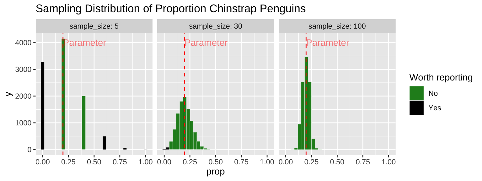
Figure 9: Comparing the sampling distribution of faculty proportion in samples of size five, thirty, and one hundred. The true population proportion is 0.198. Bars are colored by whether they are likely to be reported (less than 5% or more than 39%), with unremarkable observations in dark green.
The key takeaway here is that whenever you see an exceptional claim, be sure to look at the sample size and measures of uncertainty, which we’ll discuss in the next chapter. For a deeper dive into this issue, check out this optional reading: The Most Dangerous Equation (Wainer 2007).
Small Samples, Overestimation, and the File Drawer Problem
Let’s say you have a new and exciting idea—maybe a pharmaceutical intervention to cure a deadly cancer. Before you commit to a large-scale study, you might do a small pilot project with a limited sample size. This is a necessary step before getting the funding, permits, and time needed for a bigger study.
- What if you found an amazing result? The drug worked even better than you expected! You would likely shout it from the rooftops—issue a press release, etc.
- What if you found something subtle? The drug might have helped, but the result is inconclusive. You might keep working on it, but more likely, you’d move on to a more promising target.
After reading this section, you know that both of these outcomes could happen for two drugs with the exact same effect (see Figure 9). This combination of sampling and human nature has the unfortunate consequence that reported results are often biased toward extreme outcomes. This issue, known as the file drawer problem (because underwhelming results are kept in a drawer somewhere, waiting for a mythical day when we have time to publish them), means that reported results are often overestimated, modest effects are under-reported, and follow-up studies tend to show weaker effects than the original studies. Importantly, this happens even when experiments are performed without bias, and insisting on statistical significance doesn’t solve the problem. It is therefore exceptionally important to report all results—even boring, negative ones.
Quiz
Figure 10: The accompanying quiz link
Definitions, Notation, Equations, and Useful functions
Terms
Newly introduced terms
Standard error A measure of how far we expect our estimate to stray from the true population parameter. We quantify this as the standard deviation of the sampling distribution.
Pseudo-replication Analyzing non-independent samples as if they were independent. This results in misleading sample sizes and tarnishes statistical procedures.Review of terms from the introduction to statistics
Many of the concepts discussed in this chapter were first presented in the Introduction to Statistics and have been revisited in greater detail in this chapter.
Sample: A subset of a population – individuals we measure.
Parameter: A true measure of a population.
Estimate: A guess at a parameter that made from a finite sample. Sampling error: A deviation between parameter and estimate attributable to the finite process of sampling.
Sampling bias: A deviation between parameter and estimate attributable to non representative sampling.
Independence: Samples are independent if the probability that one individual is studied is unrelated to the probability that any other individual is studied.
Functions for sampling in R
sample(x = , size = , replace = , prob = ): Generate a sample of size size, from a vector x, with (replace = TRUE) or without (replacement = FALSE) replacement. By default the size is the length of x, sampling occurs without replacement and probabilities are equal. Change these defaults by specifying a value for the argument. For example, to have unequal sampling probabilities, include a vector of length x, in which the \(i^{th}\) entry describes the relative probability of sampling the \(i^{th}\) value in x.
slice_sample(.data, ..., n, prop, weight_by = NULL, replace = FALSE): Generate a sample of size n, from a tibble .data, with (replace = TRUE) or without (replacement = FALSE) replacement. All arguments are the same as in sample() except weight replaces prob, and .data replaces x. slice_sample() is a function in the dplyr package, which is loaded with tidyverse.