Chapter 23: 2ts

Two samples from normal distributions.

Motivating Scenario:
Suppose you want to compare the effectiveness of two different treatments, measure the average heights of two distinct plant species, or assess whether two groups of students perform differently on a test. In each of these cases, you have two samples, and your goal is to determine if there is a significant difference between their means. The two-sample t-test is the go-to test to address this type of question.

Learning Goals: By the end of this chapter, you should be able to

• Understand when and how to use a two-sample t-test.
  
• Distinguish between a paired and two-sample t-test.
  
• Work through the mathematical calculations involved in a two-sample t-test.
  
• Conduct a two sample t-test in R.
  
• State and check the assumptions required for a valid two-sample t-test.
  
• Know alternative methods to use when the assumptions of a two-sample t-test are violated.
  
• Pose a two sample t-test as a linear model.

2t example: Lizard survival

Could long spikes protect horned lizards from being killed by the loggerhead shrike? The loggerhead shrike is a small predatory bird that skewers its victims on thorns or barbed wire. Young, Brodie, and Brodie (2004) compared horns from lizards that had been killed by shrikes to 154 live horned lizards. The data are plotted below.

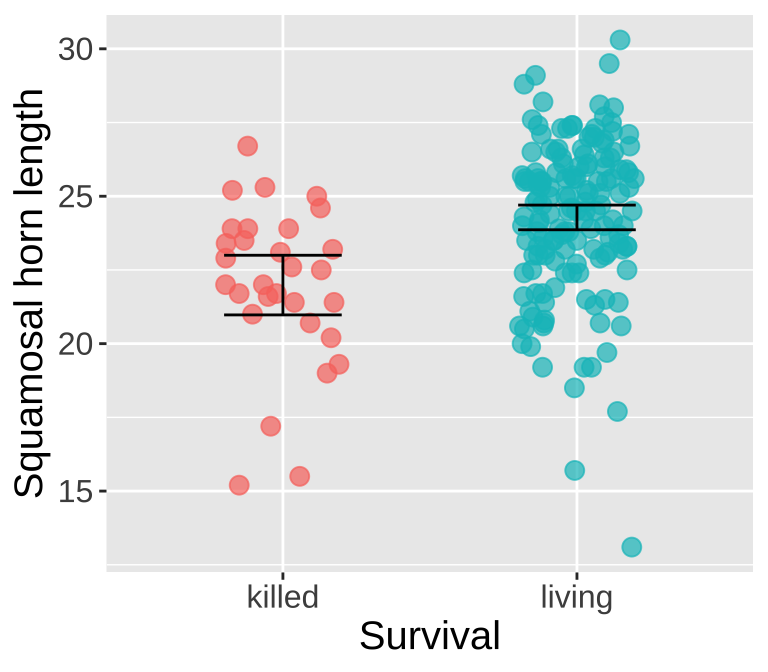
Figure 1: Squamosal horn length in living vs killed lizard. Data is available here, and is fromresearch in Young, Brodie, and Brodie (2004).

Living Lizard summary stats: From our sample of 154 living lizards, the mean horn length was 24.28, with a sample variance of 6.92.

Killed Lizard summary stats: From our sample of 30 killed lizards, the mean horn length was 22, with a sample variance of 7.34.

Summarizing the difference in Killed and Living lizards: So, surviving lizards have horns that are 2.29 longer than killed lizards.

Calculations for a Two-Sample t-Test

We can calculate the group means and the difference between these means, as well as the variances within each group. But how do we turn these into estimates of uncertainty in the between-group difference (i.e., the standard error and 95% confidence intervals)? And how can we test the null hypothesis that the groups represent samples from the same population? To begin addressing these questions, we need to compute the within-group (or pooled) variance in horn length.

The Pooled Variance

How do we think about this variance? I like to conceptualize it as: “On average, how much do we expect the square of the difference between one random individual from each group to deviate from the average difference between the groups?” The pooled variance, (\(s_p^2\)), approximates this idea. It is calculated by weighting the variance in each group by its degrees of freedom (\(df_1\)) and (\(df_2\)) and dividing by the total degrees of freedom (\(df_t = df_1 + df_2\)).

\[\begin{equation} \begin{split} s_p^2 &= \frac{df_1\times s_1^2+df_2\times s_2^2}{df_1+df_2} \end{split} \tag{1} \end{equation}\]

Calculating the Pooled Variance in the Lizard Example

Recall that we had 154 living lizards with a sample variance in horn length of 6.92 and 30 killed lizards with a sample variance of 7.34. Therefore, the pooled variance is calculated as follows:

\[\begin{equation} \begin{split} s_p^2 &= \frac{df_1\times s_1^2+df_2\times s_2^2}{df_1+df_2}\\ &= \frac{df_\text{living}\times s_\text{living}^2+df_\text{killed}\times s_\text{killed}^2}{df_\text{living}+df_\text{killed}}\\ &= \frac{(154-1)\times 6.92 + (30-1)\times 7.34}{154 + 30 -2} \\ &= 6.99 \end{split} \tag{2} \end{equation}\]

We can calculate this in R:

• First we calculate all the bits we need to find the pooled variance (i.e. the variance and deegrees of freedom in each group). I also keep track of the means as a handy value to have around:

# First, we get the summaries
lizard_summaries <- lizards %>%
  group_by(Survival) %>%
  summarise(n = n(),                        # Sample size for each group
            df = n - 1,                     # Degrees of freedom for each group
            mean_horn = mean(squamosalHornLength),  # Mean horn length for each group
            var_horn = var(squamosalHornLength))    # Variance of horn length for each group

lizard_summaries  # Check the summaries

# A tibble: 2 × 5
  Survival     n    df mean_horn var_horn
  <chr>    <int> <dbl>     <dbl>    <dbl>
1 killed      30    29      22.0     7.34
2 living     154   153      24.3     6.92

• Now, from these bits, we canc calucalte the pooled variance

# Then we calculate the pooled variance and the difference in means
lizard_summaries_2 <- lizard_summaries %>% 
  summarise(pooled_variance = sum(df * var_horn) / sum(df), # calculate the pooled variance
            mean_horn_diff = diff(mean_horn))               # calculate the difference in means

lizard_summaries_2

# A tibble: 1 × 2
  pooled_variance mean_horn_diff
            <dbl>          <dbl>
1            6.99           2.29

Effect Size of the Difference Between Killed and Living Lizards

We previously found that surviving lizards have horns that are, on average, 2.29 mm longer than those of killed lizards. To give this difference more context, we can calculate the effect size, Cohen’s d, which standardizes the difference by the pooled standard deviation. The following math shows that the average surviving lizard’s horn is about 0.87 standard deviations longer than the average killed lizard,

which is quite a substantial difference.

\[\text{Cohen's d } = \frac{\text{distance from null}}{s} = \frac{24.28 - 21.99}{\sqrt{ 6.99}} = \frac{2.29}{\sqrt{ 2.64}} = 0.87\] Recall that

• Cohen’s D from 0.0 to 0.5 is considered a small effect size.
  
• Cohen’s D from 0.5 to 0.8 is considered a medium effect size.
  
• Cohen’s D from 0.8 to 1.2 is considered a large effect size.
  
• Cohen’s D greater than 1.2 is considered very a large effect size.

As such, this Cohen’s D of 0.87 is a substantial difference.

The standard error

So Cohen’s D showed a large difference in horn lengths. But how does this difference compare to what we expect by sampling error?

We could, of course, get a sense of this sampling error by resampling from each group with replacement, and calculating the mean difference for each “bootstrapped” replicate to approximate a sampling distribution, and use this to calculate a standard error and confidence interval

lizard_boot <- replicate(n = 10000, simplify = FALSE,
  lizards %>%
  group_by( Survival)                      %>%
  slice_sample(prop = 1, replace = TRUE)   %>%
  dplyr::summarise(mean_horn = mean(squamosalHornLength)) %>%
  dplyr::summarise(mean_horn_diff = diff(mean_horn))) %>%
  bind_rows()

lizard_boot %>%
  summarise(se_mean_diff = sd(mean_horn_diff),
            lower_CI_horn_diff = quantile(mean_horn_diff, prob = 0.025),
            upper_CI_horn_diff = quantile(mean_horn_diff, prob = 0.975))

# A tibble: 1 × 3
  se_mean_diff lower_CI_horn_diff upper_CI_horn_diff
         <dbl>              <dbl>              <dbl>
1        0.530               1.31               3.36

Alternatively, we can use math tricks to estimate the standard error. Specifically, the standard error for the difference in means, \(SE_{\overline{x_1}-\overline{x_2}}\) equals \(SE_{\overline{x_1}-\overline{x_2}} = \sqrt{s_p^2 \Big(\frac{1}{n_1} + \frac{1}{n_2}\Big)}\), where \(s_p^2\) is the pooled variance from Equation (1). In this case, \(SE_{\overline{x_1}-\overline{x_2}} = \sqrt{6.99 \Big(\frac{1}{154} + \frac{1}{30}\Big)} = 0.528\).

As in our introduction to the t-distribution, we can use equation: \((1-\alpha)\%\text{ CI } = \overline{x} \pm t_{\alpha/2} \times SE_x\) – to find the upper and lower confidence intervals.

Again, we can perform these calculations in R. As shown below, the mathematical results are very close to the bootstrap-based estimates of uncertainty.

alpha <- 0.05
lizard_summaries_3 <- lizard_summaries %>% 
  summarise(est_diff        = abs(diff(mean_horn)),
            pooled_variance = sum(df * var_horn) / sum(df),
            se              = sqrt(sum(pooled_variance/n)),
            crit_t_95       = qt(p = alpha/2, df = sum(df), lower.tail = FALSE),
            lower_95CI      = est_diff  - se * crit_t_95,
            upper_95CI      = est_diff  + se * crit_t_95) 

lizard_summaries_3

# A tibble: 1 × 6
  est_diff pooled_variance    se crit_t_95 lower_95CI upper_95CI
     <dbl>           <dbl> <dbl>     <dbl>      <dbl>      <dbl>
1     2.29            6.99 0.528      1.97       1.25       3.34

We can also see that a normal distribution, with a mean equal to the estimated difference in means and a standard deviation equal to the standard error of this estimate, fits the bootstrap distribution of the difference in means remarkably well (Figure @(fig:bootvnormal))!

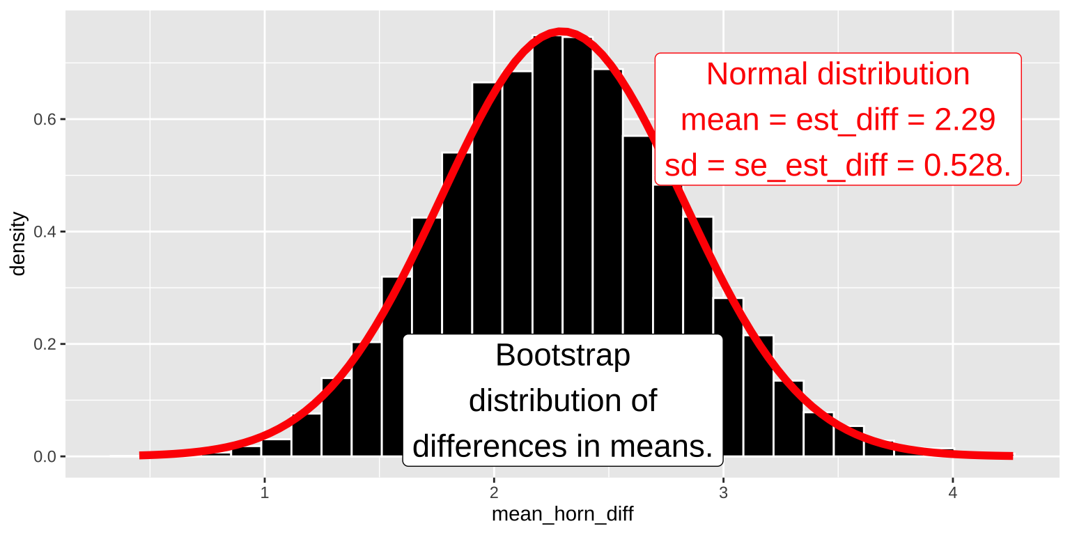
Figure 2: A comparison of the sampling distribution of the mean difference estimated by bootstrapping (shown as a histogram) to the distribution estimated by a normal curve, with the means and variances set to those calculated in this example. code here

Quantifying Surprise

How surprised would we be to see such an extreme difference if we expected no difference at all? The p-value quantifies this level of surprise.

We can estimate this by permutation:

We then find the proportion ot the permuted distribution that was as or more extreme than the observed difference:

lizard_perm %>%
  mutate(as_or_more_extreme = abs(mean_horn_diff) >=  abs(pull(lizard_summaries_2,mean_horn_diff)) ) %>%
  dplyr::summarise(p_value = mean(as_or_more_extreme))

# A tibble: 1 × 1
  p_value
    <dbl>
1 0.00002

We find a very small p-value and reject the null hypothesis.

Alternatively, we could:

• Calculate a t-value (as we did in the previous chapter).
• Compare the observed t to the t distribution with 182 degrees of freedom.
• Find the area under the curve that exceeds our observed t on either tail of the distribution.

First, we calculate the t-value as \(\frac{est - \mu_0}{se} = \frac{2.294-0}{0.5274} = 4.35\). Then, we compare it to the null sampling distribution. Figure 3 shows that the p-value is very small — we need to zoom in on the null sampling distribution to see anything as or more extreme than our test statistic.

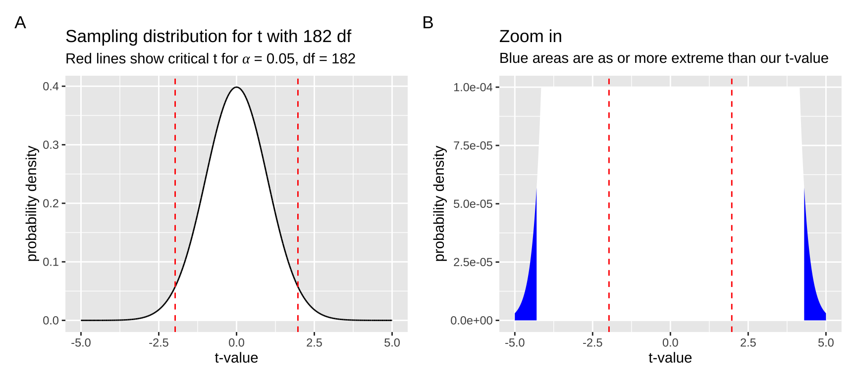
Figure 3: The null sampling distribution for t with 182 degrees of freedom. In (a), it is clear that our t-value is exceptional. Zooming in (b), we see very little of the sampling distribution is as or more extreme than our test statistic of 4.35 (blue). code here

The exact p-value is:

• 2 * pt(4.35, df = 182, lower.tail = FALSE) =
  
• \(2 \times 1.13 \times 10^{-5}\) =
  
• \(2.26 \times 10^{-5}\).

We can calculate this in R:

lizard_summaries %>% 
  summarise(est_diff        = abs(diff(mean_horn)),
            pooled_variance = sum(df * var_horn) / sum(df),
            se              = sqrt(sum(pooled_variance/n)),
            t               = est_diff / se,
            p               = 2 * pt(t, df = sum(df), lower.tail = FALSE))

# A tibble: 1 × 5
  est_diff pooled_variance    se     t         p
     <dbl>           <dbl> <dbl> <dbl>     <dbl>
1     2.29            6.99 0.528  4.35 0.0000227

A Two-Sample t-Test in R

There are several ways to conduct a two-sample t-test in R:

• By hand (as shown earlier).
• Using the t.test() function.
• Using the lm(). (later in this section).

Using the t.test() Function

First, we can use the t.test() function:

# Either of these two approaches works. 
# Note that `data = .` tells R to use the data piped in.

# lizards %>%
#    t.test(squamosalHornLength ~ Survival, data = ., var.equal = TRUE)

t.test(squamosalHornLength ~ Survival, data = lizards, var.equal = TRUE)

    Two Sample t-test

data:  squamosalHornLength by Survival
t = -4.3494, df = 182, p-value = 2.27e-05
alternative hypothesis: true difference in means between group killed and group living is not equal to 0
95 percent confidence interval:
 -3.335402 -1.253602
sample estimates:
mean in group killed mean in group living 
            21.98667             24.28117 

To make the output more compact, we can pipe it to the tidy() function in the broom package:

library(broom)    
t.test(squamosalHornLength ~ Survival, data = lizards, var.equal = TRUE) %>%
  tidy()

# A tibble: 1 × 10
  estimate estimate1 estimate2 statistic   p.value parameter conf.low
     <dbl>     <dbl>     <dbl>     <dbl>     <dbl>     <dbl>    <dbl>
1    -2.29      22.0      24.3     -4.35 0.0000227       182    -3.34
# ℹ 3 more variables: conf.high <dbl>, method <chr>,
#   alternative <chr>

Reassuringly, R’s output matches our manual calculations (though R may swap groups 1 and 2, so be mindful of that).

Assumptions

Before diving into specific assumptions, let’s take a moment to think about the role of assumptions in statistics. What exactly is an assumption? And what happens when we violate one?

An assumption is essentially a simplifying statement we make for mathematical convenience. We use them to make statistics more manageable (otherwise, we’d be dealing with custom calculations for each dataset or relying solely on bootstrapping and permutation methods).

• If our data meet the assumptions, we can be confident that the statistical methods will behave as expected.
• If the data violate assumptions, the statistics might still work—or they might not. There’s no guarantee, and definitely no refunds.

That said, many statistical tests are surprisingly robust to assumption violations (although some are not).

So, how can we tell if breaking an assumption will break our analysis, or if it’s still safe to proceed?

• The quickest way is to ask someone knowledgeable.
  
• The best way is to simulate the situation and see.

We’ll dive into simulations shortly to illustrate this point, but for now, trust me, I know.

Assumptions of the Two-Sample t-Test

The two-sample t-test assumes: Equal variance between groups, independence, normality (of residual values, or more specifically, of their sampling distribution), and unbiased data collection.

We can set aside the linearity assumption for the two-sample t-test.
While we can never ignore bias or non-independence, addressing these often requires deeper understanding of the study design. So, let’s focus on homoscedasticity (equal variances) and normality.

The Two-Sample t-Test Assumes Equal Variance Between Groups

This makes sense because we use a “pooled variance” in the two-sample t-test—essentially assuming both groups share the same variance, equal to the pooled estimate.

• Homoscedasticity means that the variance of residuals is independent of the predicted value. In the context of a two-sample t-test, where we make two predictions (one per group), this boils down to assuming equal variance in each group. We can evaluate this by checking the residuals, recalling that we’ve already calculated the variances for each group in lizard_summaries.

lizard_summaries

# A tibble: 2 × 5
  Survival     n    df mean_horn var_horn
  <chr>    <int> <dbl>     <dbl>    <dbl>
1 killed      30    29      22.0     7.34
2 living     154   153      24.3     6.92

How similar must the variances be to make a two-sample t-test valid? We’ll explore this further, but as a rule of thumb, if one group’s variance is less than five times the variance of the other, the t-test is generally robust to this assumption being violated.

The Two-Sample t-Test Assumes Normally Distributed Residuals

This means we assume the differences from the group means are normally distributed, not the raw data themselves.

As we saw with the one-sample t-test in the previous chapter, the two-sample t-test is quite robust to this assumption. In fact, we are assuming normal sampling distributions within each group, rather than a normal distribution of values across the board.

Let’s check this assumption by creating a QQ plot:

lizards %>%
    ggplot(aes(sample = squamosalHornLength)) +
    geom_qq() +
    geom_qq_line() +
    facet_wrap(~Survival) +
    labs(title = "QQ plots of lizard data by survival group")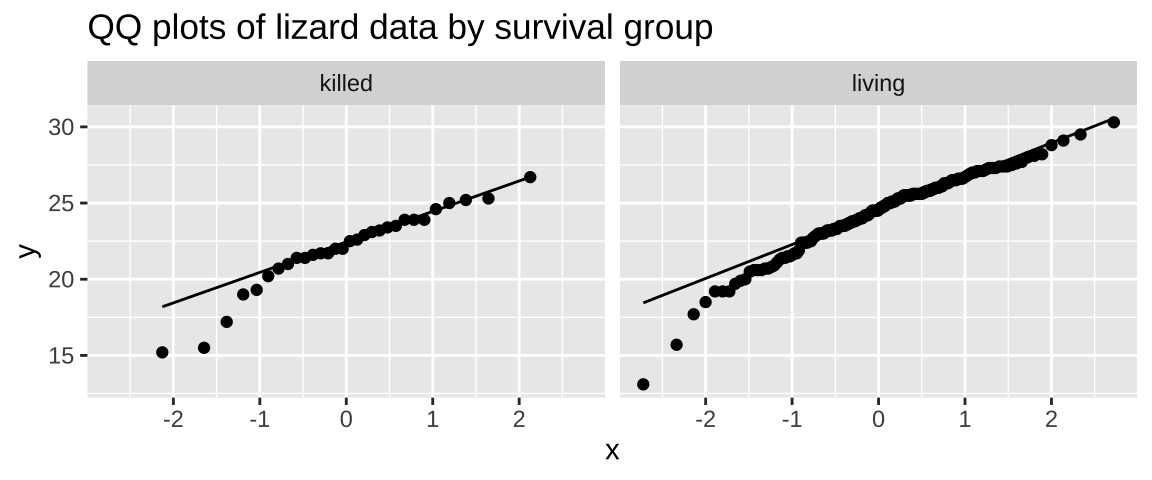

The data clearly deviate from normality, as the small values fall below the QQ line. However, given the reasonably large sample size, I’d feel comfortable assuming normality here.

Alternatives to the Two-Sample t-Test

So, what should we do if our assumptions are violated?

1. We could ignore the violation, especially if it’s minor and we believe the test is robust.
2. We could transform the data, as described in a previous chapter.
3. Or we could find a more appropriate test.

Let’s start with the third option—what alternatives do we have to the two-sample t-test?

Permutation / Bootstrapping

As discussed earlier, we can use bootstrapping (resampling with replacement) to estimate uncertainty in the mean difference, and permutation (shuffling labels) to generate a null sampling distribution for hypothesis testing.

These approaches make very few assumptions and generally work well, but they do require modest sample sizes—typically at least 15 per group—so that resampling generates enough combinations to approximate the population’s sampling distribution.

Welch’s t-Test for Unequal Variances

If group variances differ, we can perform a Welch’s t-test, which does not assume equal variance. The formula for calculating the t-value and degrees of freedom is slightly different (see below), but you don’t need to memorize it.

Just remember:

1. You can use Welch’s t-test when variances differ between groups.
   
2. In R, you can easily conduct a Welch’s t-test using the t.test() function by setting var.equal to FALSE (this is actually the default setting).

lizards %>%
  t.test(squamosalHornLength ~ Survival, data = ., var.equal = FALSE)

    Welch Two Sample t-test

data:  squamosalHornLength by Survival
t = -4.2634, df = 40.372, p-value = 0.0001178
alternative hypothesis: true difference in means between group killed and group living is not equal to 0
95 percent confidence interval:
 -3.381912 -1.207092
sample estimates:
mean in group killed mean in group living 
            21.98667             24.28117 

Interpretation of results remains the same as for the two-sample t-test:

• The t-value still represents the distance, in standard errors, between the observed difference in sample means and the null hypothesis (i.e., no difference).
• The p-value still indicates the proportion of draws from the null hypothesis that are as or more extreme than our test statistic.

The only difference is that the sampling distribution now uses the variances from each group, rather than combining them into a pooled variance.

Mann-Whitney U and Wilcoxon Rank-Sum Tests

If residuals are not normally distributed, we might use a permutation test today. Historically, though, rank-based “non-parametric” tests were employed when data weren’t normal. These tests:

• Convert data values into ranks (e.g., first, second, third, etc.).
• Use the ranks to calculate a test statistic.
• Find a null distribution for ranks.
• Calculate a p-value, and reject or fail to reject the null hypothesis.

Here’s how to run a Wilcoxon rank-sum test in R:

lizards %>%
  wilcox.test(squamosalHornLength ~ Survival, data = .)

    Wilcoxon rank sum test with continuity correction

data:  squamosalHornLength by Survival
W = 1181.5, p-value = 2.366e-05
alternative hypothesis: true location shift is not equal to 0

These rank-based tests are becoming less common, as they don’t estimate uncertainty, have their own assumptions, and bootstrapping/permutation tests are easier to run on modern computers. I include this just to familiarize you with it—you might encounter it, but we won’t focus on it here.

A two-sample t-test as a linear model

As we have previously seen, we can model differences between groups using a linear model. Recall that a linear model describes the predicted value of a response variable for the \(i^{th}\) individual, \(\hat{Y_i}\), as a function of one or more explanatory variables, where the hat denotes that this is a prediction. That is, \(\hat{Y_i} = f(\text{explanatory variables}_i)\).

Of course, model predictions will rarely match reality, and the difference between an individual’s observed value (\(Y_i\)) and predicted value (\(\hat{Y_i}\)) is the residual, \(\epsilon_i\):

\[Y_i = \hat{Y_i} + \epsilon_i\]
\[\epsilon_i = Y_i - \hat{Y_i}\]

When conducting a two-sample t-test as a linear model, our model looks like this:

\[\hat{Y_i} = a + \text{GROUP}_i \times b\]

This can be a bit tricky to understand, so I’ll walk you through it:

• \(a\) is the intercept (also known as the reference value). It represents the value of an individual before we know which group it belongs to. It also happens to be the mean of one of the two groups (the reference group).
• \(\text{GROUP}_i\) indicates which group the individual is in. It equals zero for individuals in the reference group and 1 for individuals in the other group.
• \(b\) is the difference in means between our two groups.

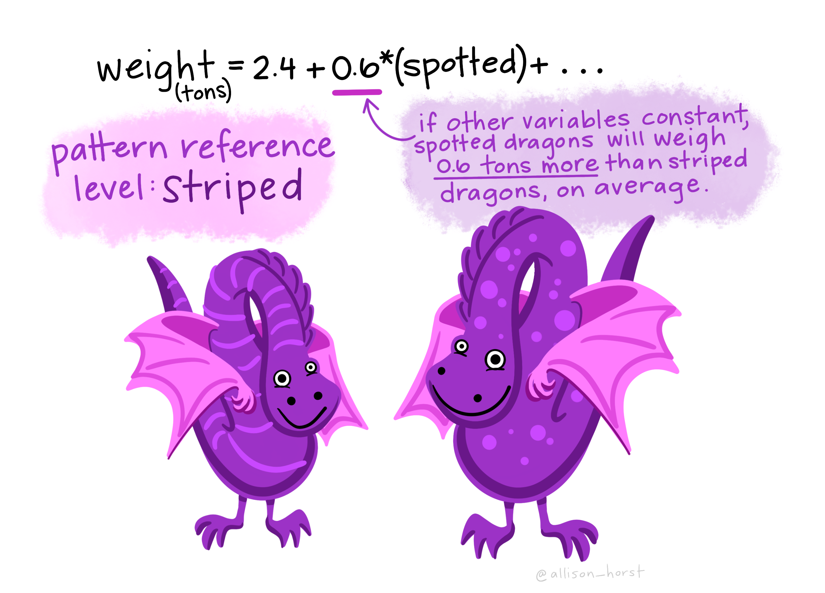
Figure 4: A cartoon of a two sample comparison as a linear model.

The lm() function in R

Let’s work through this with our lizard example using the lm() function in R:

lizard_model <- lm(squamosalHornLength ~ Survival, data = lizards)
lizard_model

Call:
lm(formula = squamosalHornLength ~ Survival, data = lizards)

Coefficients:
   (Intercept)  Survivalliving  
        21.987           2.295  

Here, the intercept \(a\) of 21.987 represents the mean squamosal horn length in killed lizards. The difference in mean horn lengths between surviving and killed lizards is indicated by the SurvivalLiving coefficient, which equals 2.295. How do we know that “killed” is the reference group? It’s because R doesn’t show a coefficient for SurvivalKilled.

So, we have our predictions for the mean squamosal horn length for both living and killed lizards:

\[\text{Expected(Squamosal Horn Length | Killed)} = 21.987 + 0 \times 2.295 = 21.987\] \[\text{Expected(Squamosal Horn Length | Living)} = 21.987 + 1 \times 2.295 = 24.282\]

Partitioning sums of squares and finding \(r^2\)

A commmon summary of a linear model is \(r^2\), the proportion of variance “explained” by our model. This is the ratio of the sum of squared differences between our predicted values and the grand mean, relative to the sum of squared differences between our observed values and the grand mean.

\[r^2 = \text{SS}_\text{model}/\text{SS}_\text{total}\] \[\text{SS}_\text{model} = \Sigma(\hat{Y_i}-\bar{Y})^2\] \[\text{SS}_\text{total} = \Sigma(Y_i-\bar{Y})^2\]

lizard_SS <- lizards %>%  
  group_by(Survival) %>%
  mutate(prediction = mean(squamosalHornLength))%>%
  ungroup()%>%
  mutate(id = 1:n()) %>%                                       # Create an 'id' column to uniquely identify each row
  mutate(
    grand_mean     = mean(squamosalHornLength),                # Calculate the grand mean of bill length
    total_error    = squamosalHornLength- grand_mean,          # Calculate the total deviation from the grand mean
    model_explains = prediction - grand_mean,                  # Calculate the deviation explained by the model
    residual_error = squamosalHornLength - prediction          # Calculate the residual error (unexplained by the model)
  )

How much variation in Squamosal Horn Length length in these lizards is explained by survival alone? The code below calculates an \(r^2\) of 0.094.

lizard_SS %>%
  summarise(SS_total = sum(total_error^2),
            SS_model = sum(model_explains^2),
            SS_error = sum(residual_error^2),
            r2       = SS_model / SS_total)

# A tibble: 1 × 4
  SS_total SS_model SS_error     r2
     <dbl>    <dbl>    <dbl>  <dbl>
1    1404.     132.    1272. 0.0942

I find this visualization helps me think about the different components of variance:

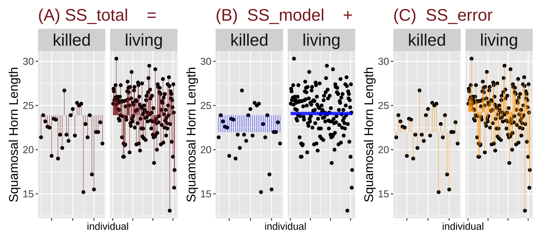
Figure 5: Partitioning the sums of squares for a model of squamosal horn length as a function of survival (code here).

Note we can also find \(r^2\) from the glance() function in the broom package!

glance(lizard_model)

# A tibble: 1 × 12
  r.squared adj.r.squared sigma statistic   p.value    df logLik   AIC
      <dbl>         <dbl> <dbl>     <dbl>     <dbl> <dbl>  <dbl> <dbl>
1    0.0942        0.0892  2.64      18.9 0.0000227     1  -439.  884.
# ℹ 4 more variables: BIC <dbl>, deviance <dbl>, df.residual <int>,
#   nobs <int>

Null Hypothesis Significance Testing of lm() Output

Now that we have an equation for our linear model fit, it’s time to estimate uncertainty and conduct null hypothesis significance testing. The first way I’ll show you is using the summary() function:

lizard_model <- lm(squamosalHornLength ~ Survival, data = lizards)
summary(lizard_model)

Call:
lm(formula = squamosalHornLength ~ Survival, data = lizards)

Residuals:
     Min       1Q   Median       3Q      Max 
-11.1812  -1.2812   0.2688   1.7188   6.0188 

Coefficients:
               Estimate Std. Error t value Pr(>|t|)    
(Intercept)     21.9867     0.4826  45.556  < 2e-16 ***
Survivalliving   2.2945     0.5275   4.349 2.27e-05 ***
---
Signif. codes:  0 '***' 0.001 '**' 0.01 '*' 0.05 '.' 0.1 ' ' 1

Residual standard error: 2.643 on 182 degrees of freedom
Multiple R-squared:  0.09415,   Adjusted R-squared:  0.08918 
F-statistic: 18.92 on 1 and 182 DF,  p-value: 2.27e-05

For now, let’s focus on the “Coefficients” section of the output. You can extract this by typing summary(lizard_model)$coefficients or using the tidy() function from the broom package:

tidy(lizard_model)

# A tibble: 2 × 5
  term           estimate std.error statistic   p.value
  <chr>             <dbl>     <dbl>     <dbl>     <dbl>
1 (Intercept)       22.0      0.483     45.6  1.90e-101
2 Survivalliving     2.29     0.528      4.35 2.27e-  5

• The estimates for the (Intercept) and Survivalliving correspond to the values we saw earlier from the linear model. The standard error summarizes the uncertainty in our estimates.
  
• The standard error for Survivalliving equals 0.528, which matches exactly what we found with the t.test() function.
  
• The statistic (which is the t-value for this model) for Survivalliving is 4.349, which is reassuringly identical to the value we obtained from the two-sample t-test.
  
• Similarly, the p-value of 0.0000227 for Survivalliving matches our previous calculations.

The statistic (i.e., the t-value) and the p-value for the (Intercept) aren’t particularly important or interesting here. The statistic describes the number of standard errors between our reference value for Squamosal Horn Length and zero. The p-value for the (Intercept) tests the null hypothesis that Squamosal Horn Length is greater than zero. Since horn lengths cannot be negative, this is a stupid null hypothesis, so we can safely ignore this part of the output.

Quiz

Figure 6: Quiz on the two-sample t-test here

Optional

Welch’s Test Math

You don’t need to memorize this, but here is the formula for Welch’s t-test:

\[t = \frac{\overline{X}_1 - \overline{X}_2}{\sqrt{\frac{s_1^2}{N_1} + \frac{s_2^2}{N_2}}}\]

With degrees of freedom approximately equal to:

\[df \approx \frac{\left(\frac{s_1^2}{N_1} + \frac{s_2^2}{N_2}\right)^2}{\frac{s_1^4}{N_1^2 \times df_1} + \frac{s_2^4}{N_2^2 \times df_2}}\]

Other Approaches When Data Do Not Meet Assumptions

Fit Your Own Likelihood Model

If you can write down a likelihood function, you can customize your assumptions to fit the data. We will discuss this approach later.

Simulations to Evaluate Test Performance

We often want to know what to expect from a statistical test. For example, we might want to:

• Evaluate how robust a test is to violations of its assumptions, or
  
• Assess the power of a test to reject a false null hypothesis.

We can do both by simulation! Here, we’ll focus on the robustness of the two-sample t-test when the assumption of equal variance is violated.

First, we set up the parameters. We’ll perform 10,000 repetitions, with the variance in group 1 always set to 1, and the variance in group 2 set to 1, 2, 5, and higher:

n_experiments_per_pair  <- 10000 
vars <- c(1, 1, 1, 2, 1, 5, 1, 10, 1, 25, 1, 50, 1, 100)
var_grp_2 <- vars[1:length(vars) %% 2 == 0]  # A trick to grab the even values

Next, we generate data for sample sizes of 10 and 50. The code below simulates data for each experiment:

• Assigns individuals to group 1 or 2,
• Ensures group 1 has a variance of 1 and group 2 has the specified variance (1, 2, 5, etc.),
• Simulates data for each individual from a normal distribution with a mean of 0 and standard deviation equal to the square root of the variance.

# Sample size of 10
n <- 10
sim_n10 <- tibble(this_var = rep(rep(vars, each = n), times = n_experiments_per_pair),
                  this_group = rep(rep(rep(1:2, each = n), times = length(var_grp_2)), times = n_experiments_per_pair),
                  this_experiment = rep(1:(n_experiments_per_pair * length(var_grp_2)), each = 2 * n),
                  var_g2 = rep(rep(var_grp_2, each = 2 * n), times = n_experiments_per_pair),
                  n = n) %>%
  mutate(sim_val = rnorm(n(), mean = 0, sd = sqrt(this_var)))

# Sample size of 50
n <- 50
sim_n50 <- tibble(this_var = rep(rep(vars, each = n), times = n_experiments_per_pair),
                  this_group = rep(rep(rep(1:2, each = n), times = length(var_grp_2)), times = n_experiments_per_pair),
                  this_experiment = rep(1:(n_experiments_per_pair * length(var_grp_2)), each = 2 * n),
                  var_g2 = rep(rep(var_grp_2, each = 2 * n), times = n_experiments_per_pair),
                  n = n) %>%
  mutate(sim_val = rnorm(n(), mean = 0, sd = sqrt(this_var)))

We then calculate the p-values for these data, simulated under a null hypothesis but breaking the assumption of equal variance:

sim_tests <- bind_rows(sim_n10, sim_n50) %>%
  group_by(this_experiment, n) %>%
  nest(data = c(this_group, this_var, sim_val)) %>%
  mutate(fit = map(data, ~ t.test(.x$sim_val ~ .x$this_group, var.equal = TRUE)),
         results = map(fit, tidy)) %>%
  unnest(results) %>%
  select(this_experiment, var_g2, n, p.value)

Finally, we assume a traditional \(\alpha = 0.05\) and calculate the proportion of times we reject the null hypothesis:

sim_summary <- sim_tests %>%
  mutate(reject = p.value <= 0.05) %>%
  group_by(n, var_g2) %>%
  summarise(actual_alpha = mean(reject)) %>%
  mutate(`Sample size` = factor(n))

ggplot(sim_summary, aes(x = var_g2, y = actual_alpha, color = `Sample size`)) +
  geom_line() +
  geom_point() +
  scale_x_continuous(trans = "log2", breaks = c(1, 2, 5, 10, 25, 50, 100)) +
  geom_hline(yintercept = 0.05) +
  labs(x = "Population variance in group 2\n(population variance in group 1 is always 1)")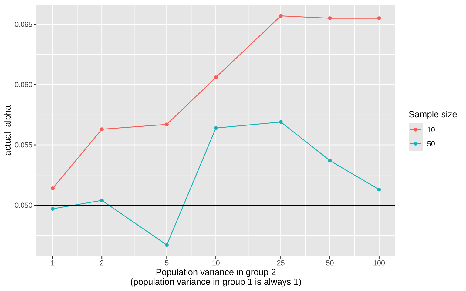

The plot shows that violating the assumption of equal variance has the greatest impact when sample size is small and the variance differences are extreme.

Definitions, Notation, and Equations

Two-sample t-test: A statistical test used to determine whether there is a significant difference between the means of two groups. The test assumes data are normally distributed and the variances are equal (i.e. homoscedasticity).

Homoscedasticity: The assumption that the variance of errors or residuals is constant across all levels of the independent variable(s) in a model. In a two-sample t-test, this means the variance does not differ between groups.

Wilcoxon rank-sum test (Mann-Whitney U test): A non-parametric alternative to the t-test, used to compare two independent samples when the assumption of normality is violated. It ranks data from both samples and compares these ranks between the two groups.

Test statistic: A standardized value that is calculated from sample data during a hypothesis test. For a t-test, this is the t-statistic.

Confidence interval (CI): A range of values, derived from the sample data, that is likely to contain the population parameter (such as the mean) with a specified level of confidence.

Null hypothesis (H₀): A statement that there is no effect or no difference, used as the default or starting assumption in hypothesis testing.

Alternative hypothesis (H₁ or Hₐ): A statement that contradicts the null hypothesis, suggesting there is an effect or a difference.

p-value: The probability of obtaining a test statistic at least as extreme as the one observed, under the assumption that the null hypothesis is true. We reject the null hypothesis when p is less than alpha (usually 0.05).

Degrees of freedom (df): The number of independent values or quantities that can vary in a statistical calculation. In a t-test, df is related to the sample size.

Effect size: A quantitative measure of the magnitude of the experimental effect, typically used in conjunction with p-values to assess the practical significance of results.

R Functions for Two-Sample Tests

Summary and Model Functions
summary(): Provides a summary of various R objects, giving key descriptive statistics or details depending on the object type. When used on an lm object, it returns model coefficients, residual summaries, R-squared values, and significance tests for the fitted linear model.

lm(): Fits a linear model to data. Can also be used for comparing means between groups when coupled with a two-sample t-test.
tidy(): Provides a tidy summary of model outputs, turning model coefficients into a tibble.
glance(): Provides a one-row summary of model fit statistics like R-squared and AIC.

Hypothesis Testing Functions
t.test(): Performs a t-test to compare the means of two independent groups, assuming normal distribution and homogeneity of variance.
wilcox.test(): Performs the Wilcoxon rank-sum test, a non-parametric alternative to the t-test for comparing two independent samples without assuming normality.

Key Equations

Here are the core equations used in this chapter for hypothesis testing:

1. Two-Sample t-Test Formula \[ t = \frac{\overline{X}_1 - \overline{X}_2}{\sqrt{s_p^2 \left(\frac{1}{n_1} + \frac{1}{n_2}\right)}} \] where:

   • \(\overline{X}_1\) and \(\overline{X}_2\) are the sample means,
   • \(s_p^2\) is the pooled variance,
   • \(n_1\) and \(n_2\) are the sample sizes.

2. Pooled Variance Formula \[ s_p^2 = \frac{(n_1 - 1) s_1^2 + (n_2 - 1) s_2^2}{n_1 + n_2 - 2} \] where \(s_1^2\) and \(s_2^2\) are the sample variances for the two groups.

3. Confidence Interval for Two-Sample t-Test \[ CI = (\overline{X}_1 - \overline{X}_2) \pm t_{\alpha/2, df} \times \sqrt{s_p^2 \left(\frac{1}{n_1} + \frac{1}{n_2}\right)} \] where \(t_{\alpha/2, df}\) is the critical t-value at a given confidence level.