Motivating Scenarios:
We want to understand how seemingly important patterns can arise by chance, how to think about chance events, how to quantify chance events, and to gain an appreciation for a foundational concern of statistics—along with how the field addresses this concern.
Learning Goals: By the end of this chapter, you should be able to:
- Provide a working definition of probability.
- Explain why we need to consider probability when interpreting data.
- Understand a proportion as an estimate of a population parameter resulting from a random outcome.
- Recognize that “random” does not mean “no clue.”
- Understand conditional probabilities and non-independence.
Why do we care about probability?
Many statistics textbooks, including ours, begin with a chapter on probability before diving into the core of statistics. But why is that? Why do I keep this chapter here (as you know from class - I’ve been waffling on this)? For me, there are three important and interrelated reasons to think about probability before getting too deep into statistics:
Many important biological processes are influenced by chance.
In my field of genetics, we know that mutation, recombination, and which grandparental allele you inherit are all chance events. Whether you get a transmissible disease after modest exposure is also a chance event. Even seemingly coordinated and predictable gene expression patterns can arise from many chance events. It’s crucial, then, to develop an intuition for how chance (random) events occur.
While it’s philosophically fun to consider whether these events are truly random, predestined, or predictable with enough information, this isn’t particularly useful. Regardless of whether something is predestined, we can only make probabilistic statements based on the information we have.We don’t want to base biological stories on coincidences.
A key lesson from probability theory is that some outcome will always happen. For every coincidence in the This American Life podcast, there are countless cases where nothing interesting happened. For example, no one called the show to report that their grandmother wasn’t in a random picture a friend sent them (No coincidence, no story). Similarly, we shouldn’t conclude that COVID restores lactose tolerance just because someone in our social circle lost their intolerance after recovering from it. Much of statistics is built on probability theory, which helps us determine whether our observations are significant or just coincidences.Understanding probability helps us interpret statistical results.
Concepts like confidence intervals, sampling distributions, and p-values are notoriously confusing. Some of that confusion comes from the complexity of the topics, but a large part comes from encountering these terms without a foundation in probability. A basic understanding of probability helps clarify statistical concepts and explain many surprising or concerning observations in scientific literature. For example, we’ll see later in this course that replication attempts often fail, and the effect of a treatment tends to shrink the longer it is studied. Understanding a bit of probability and how science works can explain these patterns.
Fortunately, none of this requires deep expertise in probability theory—though I highly recommend taking more courses in it because it’s so much fun! A quick primer, like the one we’re working through, can be quite powerful.
The most important takeaway is that random does not mean equal probability, and it certainly does not mean we have no clue. In fact, we can often make very good predictions about the world by understanding how probability works.
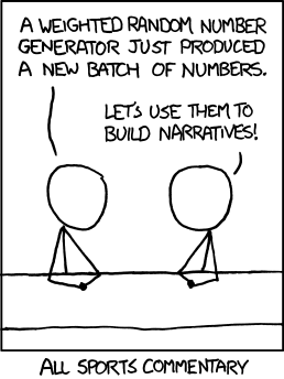
Figure 1: Comic from xkcd. Title text: Also, all financial analysis. And, more directly, D&D
Probability Concepts
Sample Space
When thinking about probability, the first step is to lay out all potential outcomes, which is formally known as the sample space.
A simple and common example of a sample space is the outcome of a coin flip, where the possible outcomes are:

Figure 2: The result of a coin flip is a classic example of a probabilistic outcome.
- The coin lands heads up.
- The coin lands tails up.
However, probabilistic events can involve more than two potential outcomes and are not always 50:50.
Consider the example of a ball dropping in Figure 3. The sample space is:
- The ball can fall into the orange bin (A).
- The ball can fall into the green bin (B).
- The ball can fall into the blue bin (C).
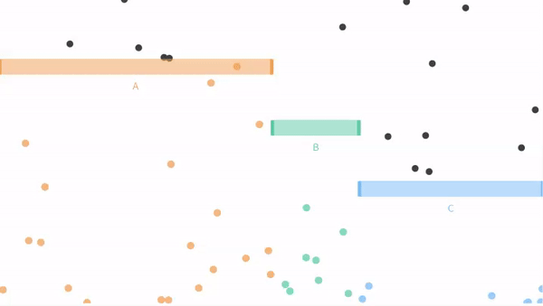
Figure 3: An example of a probability scenario from Seeing Theory (gif on 8.5 second loop). Here, outcomes A, B, and C are mutually exclusive and make up the entire sample space.
This view of probability establishes two simple truths:
- Once you lay out the sample space, some outcome is going to happen.
- As a result, the probabilities of all outcomes in the sample space will sum to one.
Point (1) helps us interpret coincidences: something had to happen (e.g., the person in the background of a photo had to be someone…), but we pay more attention when the outcome holds special significance (e.g., that person was my grandmother).
Probabilities and Proportions
Probabilities
A probability describes a parameter for a population. So, in our example, if we were to watch the balls drop indefinitely and count the proportions for each outcome, we would have the true population parameter. Alternatively, assuming that the balls fall with equal probability across the line (which they do), we can estimate the probabilities by the proportion of space each bin takes up in Figure 3. We observe that A takes up half of the sample space, B takes up 1/6 of the sample space, and C takes up about 2/6 of the sample space.
Thus, the probability of a given event P(event) is:
- P(A) = 3/6.
- P(B) = 1/6.
- P(C) = 2/6.
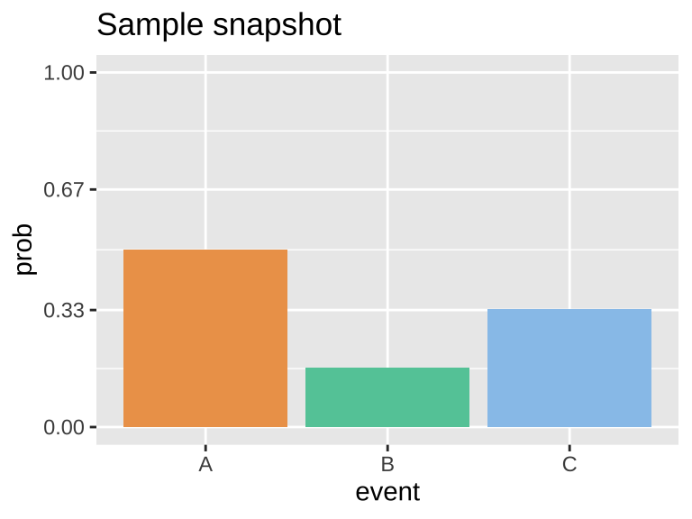
Figure 4: The probability distribution for the dropping balls example in Figure 12.1. Any probability distribution must sum to one. Strictly speaking, categorical and discrete variables can have probability distributions. Continuous variables have probability densities because the probability of observing any specific number is approximately zero. So probability densities integrate to one.
Proportions
The proportion of each outcome is the number of times we observe that outcome divided by the total number of outcomes observed. In other words, the proportion describes an estimate from a sample. Let’s look at a snapshot of a single point in time from Figure 3:

Figure 5: A still image from Figure 3. This shows ten orange two green and three blue balls.
Figure 5 shows 15 balls: 10 orange (A), 2 green (B), and 3 blue (C).
Here, the proportion of:
- A = 10/15 = 2/3 = \(0.66\overline{66}\).
- B = 2/15 = \(0.13\overline{33}\).
- C = 3/15 = 1/5 = \(0.20\).
Note that these proportions (which are estimates from a sample) differ from the probabilities (the true population parameters) due to sampling error.
Exclusive vs Non-Exclusive Events
When a coin is flipped, it will either land heads up or tails up—it cannot land on both sides at once. Outcomes that cannot occur simultaneously are called mutually exclusive.
For example, if we find a coin on the ground, it could either be heads up or tails up (mutually exclusive). Similarly, it could be a penny, nickel, dime, quarter, etc., but it cannot be all of these at once, so these outcomes are also mutually exclusive.
However, a coin can be both heads up and a quarter. These are non-exclusive events. Non-exclusive events occur when the outcome of one event does not prevent the occurrence of another.
Exclusive Events
Sticking with the coin-flipping idea, let’s use the app from Seeing Theory below to explore the outcomes of one or more exclusive events:
- Change the underlying probabilities from 50:50 (so the coin toss is unfair).
- Toss the coin once.
- Toss the coin again, repeating four times.
- Finally, toss the coin one hundred times.
Be sure to note the probabilities you chose, the outcomes of the first five tosses, and the proportion of heads and tails across all coin flips.
Non-Exclusive Events
In Figure 3, the balls falling through A, B, and C were mutually exclusive—a ball could not fall through both A and B, meaning all options were mutually exclusive.
However, this does not always have to be the case. Outcomes can be non-exclusive (e.g., if the bars were arranged so that a ball could fall through A and then through B).
Figure 6 shows an example where falling through A and B are not mutually exclusive.
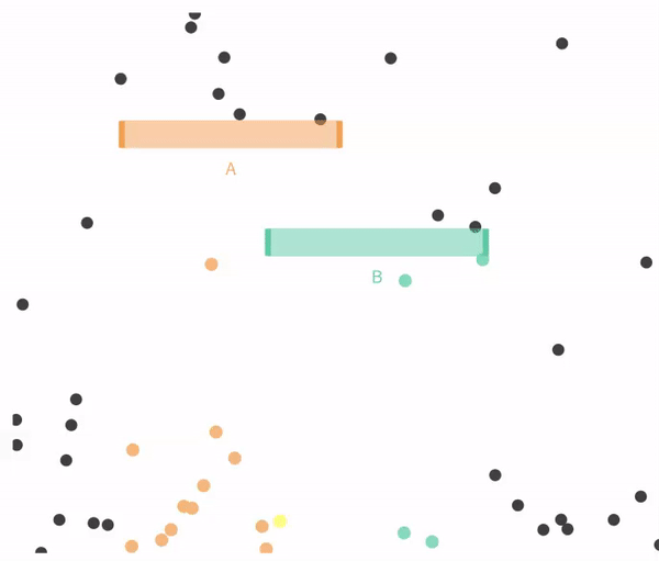
Figure 6: Non-exclusive events: Balls can go through A, B, both, or neither.
Conditional Probabilities and (Non-)Independence
Conditional probabilities help us make use of the information we already have about our system. For instance, the probability of rain tomorrow in general is likely lower than the probability of rain tomorrow given that today is cloudy. This latter probability is conditional because it incorporates relevant information.
Mathematically, calculating a conditional probability means reducing our sample space to a specific event. In the rain example, instead of considering how often it rains in general, we focus only on days when the previous day was cloudy, then check how often it rains on those days.
In mathematical notation, the | symbol represents conditional probability. For example, \(P(A|C)=0\) means that if we know outcome C occurred, then there’s no chance that outcome A also occurred. In other words, A and C are mutually exclusive.
For some unfortunate reason,
| means or in R,
but it means “conditional on” in statistics.
Stay safe.
Independent Events
Events are independent if knowing one event doesn’t provide any information about the other. Figure 7 shows a situation identical to 6, but with conditional probabilities displayed. In this example, the probability of A remains the same whether or not the ball goes through B, and vice versa.
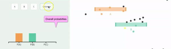
Figure 7: Conditional independence. These probabilities are identical to those in the figure above. We can reveal the conditional probabilities for all outcomes by clicking on the outcome we’re conditioning on (e.g., after clicking on B, we see P(A|B), and that P(B|B) = 1). Here, A and B are independent. That is, P(A|B) = P(A) and P(B|A) = P(B). Explore further on the Seeing Theory website.
Non-Independence
Events are non-independent if their conditional probabilities differ from their unconditional probabilities. We’ve already seen an example of non-independence. If events A and B are mutually exclusive, \(P(A|B) = P(B|A) = 0\), and \(P(A|B) \neq P(A)\), \(P(B|A) \neq P(B)\).
Understanding independence vs. non-independence is key for both basic biology and its applications. Consider a scenario where a vaccine is given, and some people get sick with another illness. If these events were independent (i.e., the proportion of sick people is similar in both vaccinated and unvaccinated groups), we’d feel fine about mass vaccination. However, if there’s a higher rate of sickness among the vaccinated group, we’d be more concerned. That said, non-independence doesn’t necessarily mean a causal link. For example, vaccinated people might socialize more, increasing their exposure to the other illness. We’d want to disentangle correlation and causation before jumping to any conclusions.
Figure 8 demonstrates non-independence:
The probability of A, P(A) = \(\frac{1}{3}\).
The conditional probability of A given B, P(A|B) = \(\frac{1}{4}\).
The probability of B, P(B) = \(\frac{2}{3}\).
The conditional probability of B given A, P(B|A) = \(\frac{1}{2}\).
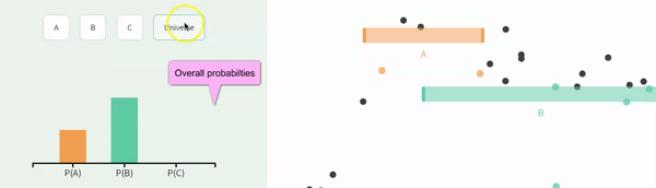
Figure 8: Non-independence: Our understanding of the likelihood that the ball fell through A changes if we know it fell through B, and vice versa, indicating non-independence. We can reveal conditional probabilities by clicking on the outcome we’re conditioning on (e.g., clicking on B shows P(A|B). Explore further on the Seeing Theory website.
Probability Rules
I strongly recommend taking a formal probability course (it was one of my favorite classes), which would dive deep into various methods for calculating probabilities of different outcomes. But for our purposes here, we don’t need to get into that level of detail. Our goal is to develop an intuition for probability by understanding a few key, straightforward rules.
If you internalize these simple rules, you’ll be in good shape:
- Add probabilities to calculate the likelihood of one outcome OR another (but remember to subtract any double-counting).
- Multiply probabilities to calculate the likelihood of one outcome AND another (and account for conditional probabilities if the events are non-independent).
Alright, let’s break down these rules step by step.
Adding Probabilities for OR Statements
To find the probability of one event OR another, we add up all the possible ways the events can happen, making sure to avoid double-counting.
\[\begin{equation} \begin{split} P(a\text{ or }b) &= P(a) + P(b) - P(ab)\\ \end{split} \tag{1} \end{equation}\]
where \(P(ab)\) is the probability of both a and b happening together.
Special Case: Mutually Exclusive Outcomes
When outcomes are mutually exclusive, the probability of both happening is zero, so \(P(ab) = 0\). This simplifies the formula:
\[\begin{equation} \begin{split}P(a\text{ or }b | P(ab)=0) &= P(a) + P(b) - P(ab)\\ &= P(a) + P(b) - 0\\ &= P(a) + P(b) \end{split} \end{equation}\]
In the example below from Figure 3, we see that:
- P(A) = 3/6
- P(B) = 1/6
- P(C) = 2/6
Thus, the probability that the ball goes through A OR B
3/6 + 1/6 = 4/6 = 2/3.
We often use this rule to find the probability of a range of outcomes for discrete variables (e.g. the probability that the sum of two dice rolls is between six and eight = P(6) + P(7) + P(8)). This rule is often used when calculating probabilities over a range of discrete outcomes, such as the sum of dice rolls.
General Case
More generally, the probability of outcome a or b is P(a) + P(b) - P(a b) [Equation (1)]. This subtraction (which is irrelevant for exclusive events, because in that case \(P(ab) = 0\)) avoids double counting.
Why do we subtract P(a and b) from P(a) + P(b) to find P(a or b)? Figure 9 shows that this subtraction prevents double-counting – the sum of falling through A or B is \(0.50 + 0.75 = 1.25\). Since probabilities cannot exceed one, we know this is foolish – but we must subtract to avoid double counting even when the sum of probabilities do not exceed one.
 (gif on 6 second loop).](images/dontdoublecount.gif)
Figure 9: Subtract P(ab) to avoid double counting: Another example of probability example from Seeing Theory (gif on 6 second loop).
Following equation (1) and estimating that about 35% of balls falls through A and B, we find that
P(A or B) = P(A) + P(B) - P(AB)
P(A or B) = 0.50 + 0.75 - 0.35
P(A or B) = 0.90.
For a simple and concrete example, the probability a random student played soccer or ran track in high school, is the probability they played soccer plus the probability they ran track minus the probability they played soccer and ran track.
The Probability of “Not”
My favorite thing about probabilities is that they have to sum (or integrate) to one. This helps us be sure we laid out sample space right, and allows us to check our math. It also provides us with nice math tricks.
Because probabilities sum to one, the probability of “not a” equals 1 - the probability of a. This simple trick often makes hard problems a lot easier.
Multiplying Probabilities for AND Statements
The probability of two events both occurring (e.g., a and b) is found by multiplying the probability of a by the conditional probability of b given a. This can also be done in reverse:
\[\begin{equation} \begin{split} P(ab) &= P(a) \times P(b|a)\\ & = P(b) \times P(a|b) \end{split} \tag{2} \end{equation}\]
Special Cases of AND
Mutually exclusive outcomes: If two outcomes cannot both occur, the conditional probability is zero, \(P(b|a) = 0\), so \(P(ab) = 0\).
Independent outcomes: If two outcomes are independent, the probability of one given the other is simply the overall probability of the second event. For independent outcomes, \(P(b|a) = P(b)\), and so the combined probability is the product of their individual probabilities, \(P(a) \times P(b)\).
Figure 10: A Punnett Square is a classic example of independent probabilities (Image from the Oklahoma Science Project).
The Punnett square is a classic example of independent probabilities in genetics as the sperm genotype usually does not impact meiosis in eggs (but see my paper (Brandvain and Coop 2015) about exceptions and the consequences for fun). If we cross two heterozygotes, each transmits their recessive allele with probability \(1/2\), so the probability of being homozygous for the recessive allele when both parents are heterozygous is \(\frac{1}{2}\times \frac{1}{2} = \frac{1}{4}\).
General Case of AND
When outcomes are not independent, we calculate the probability of both events by multiplying the probability of one event by the conditional probability of the other event. For example, the general formula is:
\[ P(ab) = P(a) \times P(b|a) \]
Conditional Probability Visual
Here’s an example:
Figure 11: A visual representation of conditional probabilities. On the left side, alternating bar plots display the unconditional probabilities of A (P(A) = 1/3) and B (P(B=2/3)), followed by P(B|A), and then P(A|B). On the right side, a simulation shows balls passing through gates A and B—first for the entire sample space, then conditioned on A, and finally conditioned on B.
Figure 11, above, explicitly keeps track of two events:
- A (which occurs with probability P(A) = 1/3) and
- B (which occurs with probability P(B) = 2/3.
Figure 11 also shows that that the probability of A given B occuring:
- P(A|B) = 1/4,
and the probability of B given A occuring:
- P(B|A) = 1/2.
The entire sample space consists of four options
- Both A and B: We find this using Equation (2).
- P(AB) = P(A) \(\times\) P(B|A) =1/3 \(\times\) 1/2 = 1/6.
This can also be derived by flipping A and B:
- P(AB) = P(B) \(\times\) P(A| B) = 2/3 \(\times\) 1/4 = 2/12= 1/6.
- P(AB) = P(A) \(\times\) P(B|A) =1/3 \(\times\) 1/2 = 1/6.
- Only A: We find the probability of Only A as the probability of A minus the probability of Both A and B. So with a little math: P(A and not B) = P(A) - P(AB) = 1/3 - 1/6 = 1/6.
- Only B: We find the probability of Only B as the probability of B minus the probability of Both A and B. So with a little math: P(B and not A) = P(B) - P(AB) = 2/3 - 1/6 = 3/6.
- Not A and not B: We can use the rule of not to find this. P(not A and not B) = 1 - P(Only A) - P(Only B) - P(A and B). =
Using Equation (2), we find the probability of A and B:
P(AB) = P(A) \(\times\) P(B|A) = P(A) = 1/3 \(\times\) 1/2 = 1/6.
Which is the same as
P(AB) = P(B) \(\times\) P(A| B) = 2/3 \(\times\) 1/4 = 2/12= 1/6.
We can see this visually in Figure 12:
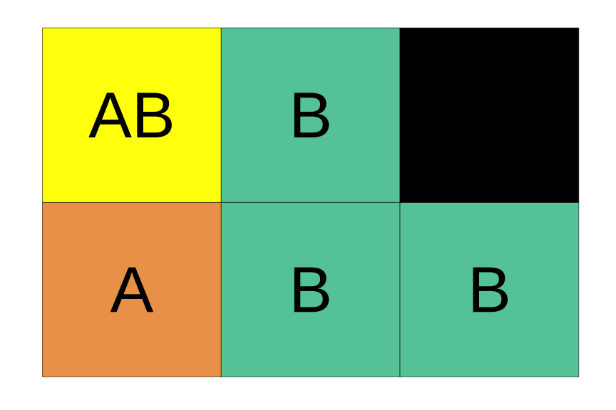
Figure 12: A representation of the relative probabilities of each outcome in sample space. Color denotes outcome (which is also noted with black letters), and each box represents a probability of one sixth.
CONDITIONAL PROBABILITY REAL WORLD EXAMPLE:
Getting a flu vaccine significantly reduces your chances of contracting the flu. But what’s the probability that a randomly selected person both got the flu vaccine and still contracted the flu? Let’s break it down with some rough probabilities:

Every year, a little more than half of the population gets a flu vaccine, let us say P(No Vaccine) = 0.58.
About 30% of people who do not get the vaccine get the flu, P(Flu|No Vaccine) = 0.30.
The probability of getting the flu diminishes by about one-fourth among the vaccinated, P(Flu|Vaccine) = 0.075.
But we seem stuck, what is \(P(\text{Vaccine})\)? We can find this as \(1 - P(\text{no vaccine}) = 1 - 0.58 = 0.42\).
Now we find P(Flu and Vaccine) as P(Vaccine) x P(Flu | Vaccine) = 0.42 x 0.075 = 0.0315.
The law of total probability
Let’s say we wanted to know the probability that someone caught the flu. How do we find this?
As discussed above, the probability of all outcomes in sample space has to sum to one. Likewise, the probability of all ways to get some outcome have to sum to the probability of getting that outcome:
\[\begin{equation} P(b) = \sum P(a_i) \times P(b|a_i) \tag{3} \end{equation}\]
The \(\sum\) sign notes that we are going over all possible outcomes of \(a\), and the subscript, \(_i\), indexes these potential outcomes of \(a\). In plain language, we find probability of some outcome by
- Writing down all the ways we can get it,
- Finding the probability of each of these ways,
- Adding them all up.
So for our flu example, the probability of having the flu is the probability of being vaccinated and having the flu, plus the probability of not being vaccinated and catching the flu (NOTE: We don’t subtract anything off because they are mutually exclusive.). We can find each following the general multiplication principle (2):
\[\begin{equation} \begin{split} P(\text{Flu}) &= P(\text{Vaccine}) \times P(\text{Flu}|\text{Vaccine})\\ &\text{ }+ P(\text{No Vaccine}) \times P(\text{Flu}|\text{No Vaccine}) \\ &= 0.42 \times 0.075 + 0.58 \times 0.30\\ &= 0.0315 + 0.174\\ &= 0.2055 \end{split} \end{equation}\]
Probability trees
It can be hard to keep track of all of this. Probability trees are a tool we use to help. To make a probability tree, we
- Write down all potential outcomes for a, and use lines to show their probabilities.
- We then write down all potential outcomes for b separately for each potential a, and connect each a to these outcomes with a line denoting the conditional probabilities.
- Keep going for events c, d, etc…
- Multiply each value on path to get the probability of that path (The general multiplication rule, Equation (2)).
- Add up all paths that lead to the outcome you are interested in. (NOTE: Again, reach path is exclusive, so we don’t subtract anything.)
Figrue 13 below, is a probability tree I drew for the flu example. Reassuringly the probability of getting the flu matches our math above.
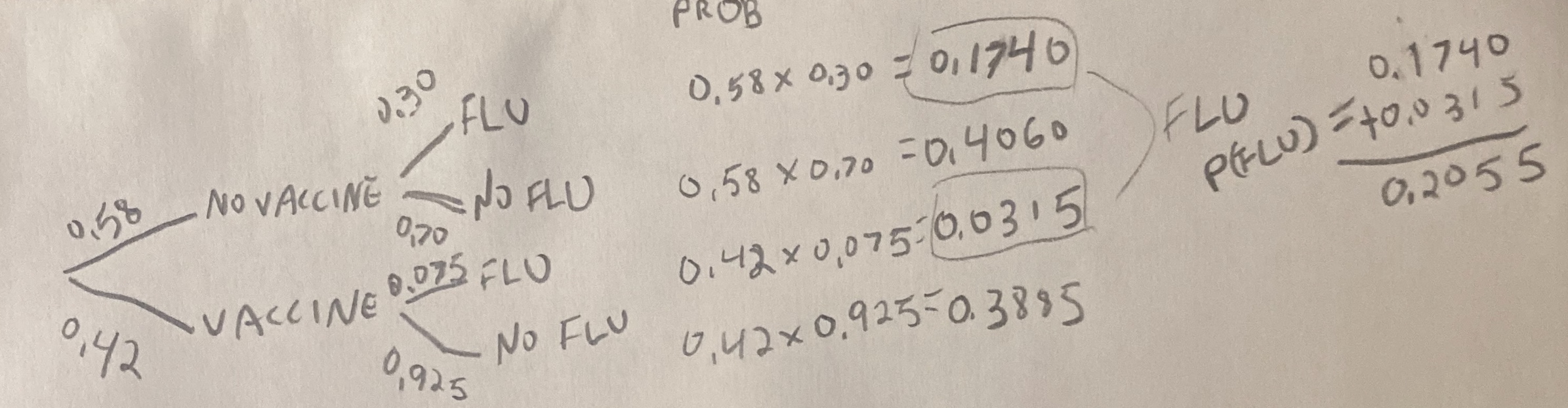
Figure 13: A probability tree illustrating the likelihood of getting the flu based on vaccination status. The tree starts with two branches: one for those who do not receive the vaccine (58%) and one for those who do (42%). Conditional probabilities are displayed for each group, showing the chance of getting the flu or not. For those unvaccinated, the probability of contracting the flu is 30%, while for those vaccinated, it drops to 7.5%. The probabilities along each path are multiplied to find the joint probability of each outcome, and the total probability of getting the flu is calculated as P(Flu) = 0.2055).
Flipping conditional probabilities
The probability that a vaccinated person gets the flu, P(Flu|Vaccine) is 0.075. But what is the probability that someone who has the flu was vaccinated, P(Vaccine|Flu)?
To understand this, we need to find the number of people who are both vaccinated and got the flu, and then divide by the total number of people who got the flu. By converting this into probabilities and using probability rules, we can express this mathematically. Specifically, the probability that someone who has the flu was vaccinated is the probability that someone was both vaccinated and got the flu, divided by the probability that someone has the flu.
\[\begin{equation} \begin{split} P(\text{Vaccine|Flu}) &= P(\text{Vaccine and Flu}) / P(\text{Flu}) \\ P(\text{Vaccine|Flu}) &= \tfrac{P(\text{Flu|Vaccine}) \times P(\text{Vaccine})}{P(\text{Vaccine}) \times P(\text{Flu}|\text{Vaccine}) + P(\text{No Vaccine}) \times P(\text{Flu}|\text{No Vaccine})}\\ P(\text{Vaccine|Flu}) &= 0.0315 / 0.2055 \\ P(\text{Vaccine|Flu}) &=0.1533 \end{split} \end{equation}\]
So, while 42% of the population is vaccinated, only 15% of those who got the flu were vaccinated.
The numerator on the right-hand side, \(P(\text{Vaccine and Flu})\), comes from the general multiplication rule (Eq. (2)).
The denominator, \(P(\text{Flu})\), comes from the law of total probability (Eq. (3)).
This is an application of Bayes’ Theorem. Bayes’ theorem allows us to “flip” conditional probabilities as follows:
\[\begin{equation} P(A|B) = \frac{P(A\text{ and }B)}{P(B)} = \frac{P(B|A) \times P(A)}{P(B)}= \frac{P(B|A) \times P(A)}{\sum P(a_i) \times P(b|a_i)} \tag{4} \end{equation}\]
Figure 14: The accompanying quiz link