Motivating scenario: Often data are not independent. For example, numerous plants may come from the same field, fish from the same lakes, or students come from the same class. If we were specifically interested in the impact of a given field, lake, or school, we could include this as a “fixed effect,” as in an ANCOVA. However, this focuses on specific fields, lakes, or schools rather than the variability among them, which is often our primary interest. Practically, we may not have enough levels (e.g., fields or lakes) to reliably estimate their effects as fixed, and this limitation sometimes makes it impossible to estimate the effect of a variable that differs across groups due to insufficient replication within groups. Random effects, by contrast, treat group-level differences as coming from a shared distribution rather than estimating them individually (that is we model the variance among groups, rather than the means of each group). This approach pools information across groups, enabling us to estimate overall effects while accounting for variability. Thus, in some cases, random effects models provide a more appropriate way to model non-independence than “fixed effects” models.
Review
Linear Models
Linear models predict \(Y\) as a deviation from some constant, \(a\), as a function of a bunch of stuff:
\[\widehat{Y_i} = a + b_1 \times y_{1,i} + b_2 \times y_{2,i} + \dots\]
Biology Breaks Assumptions of Linear Models
Linear models assume (1) data points are independent, (2) unbiased, (3) can be modeled as a linear combination of predictors, with (4) error having a mean and variance independent of predictors (5) and normally distributed.
In the previous chapter we introduced the Generalized Linear Model as an approach to model non-normal data (e.g. binomial and count data using logistic and Poisson regression). In this chapter we focus on modelling data that the assumption independence. This is important, as both nature and experimetns break the assumptions of independence.
Intro to Random Effects
In biology, we are often more interested in variability than specific individuals. For example, understanding genetic variability is critical to predicting how a population responds to natural selection. Similarly, we might care about how repeatable a trait is—if we measure the same individual twice, how similar are those measurements compared to variability in the broader sample?
Sometimes, we don’t care about the variability itself but need to account for it because it makes our data non-independent. For example, plants in the same plot may respond similarly to fertilizer due to shared conditions. In all these cases, we aren’t focused on specific individuals or locations but on understanding the variability across them. Random effects models let us capture this variability while accounting for non-independence.
Fixed vs random effects
Up to this point we have considered “fixed effects” e.g. fertilizer choice, experimental treatment etc… For these cases, we want to predict the effects of these treatments, and we don’t generalize to other treatments – for example if I looked at how three fertilizers of interest impacted plant growth, I wouldn’t go and predict the effect of a totally different fertilizer I hadn’t seen before.
However, in the examples above, we did not care about the “fixed effect”. Rather, we were interested in random effects the variability we find across “random” individuals (or locations etc.) in our population. For these cases, we don’t aim to predict the value of individuals, but rather we aim to describe the expected variability we expect across random individuals in our population. Thus, we hope to generalize to a larger population of sample units.
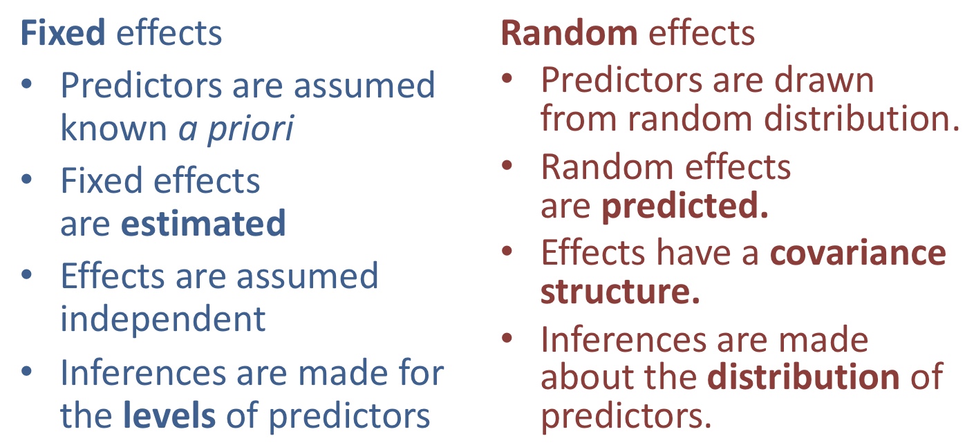
How do we know if we have a fixed or random effect?
Some is inherent to the experimental design:
- Are levels of a predictor chosen intentionally (e.g. temperature treatments)? Fixed
- Do we want to make inferences about the levels of a predictor (e.g. mean separation)? Fixed
- Can we reasonably expect covariance between levels of a predictor? Random
Some of this is inherent to the predictor:
- Are the levels of a predictor sampled from some distribution of possible levels? Random
- Can we borrow information across levels of a predictor? Random

Analysis of Variance (ANOVA)
When we work with “fixed effects,” we can test for the significance of factors in a linear model using an ANOVA framework. We previously saw that the total variance among groups includes two components: variance attributable to true differences between groups and variance attributable to random sampling error.
In an ANOVA, both of these components contribute to the mean square for groups (\(MS_{\text{groups}}\)). However, we expect that the variance caused by random sampling alone will be roughly equal to the mean square for error (\(MS_{\text{error}}\)). This is why we test the one-tailed null hypothesis that the \(F\)-statistic (calculated as \(F = \frac{MS_{\text{groups}}}{MS_{\text{error}}}\)) equals one. This corresponds to asking whether the variance among groups is greater than expected by chance, i.e., whether the true variance among groups is non-zero.
Modeling Random Effects
When modeling random effects, we take a slightly different approach than the one used in ANOVA. Instead of testing whether fixed factors explain variation, we focus on modeling the variance among the categories of our random effect. In other words, we aim to estimate how much of the total variance in the response is due to differences among groups (e.g., fields, lakes, or plots) rather than treating these groups as fixed levels of a factor.
This approach allows us to partition variance into components attributable to group-level differences and residual error. By doing so, we can account for non-independence in our data and make inferences about the population of groups, rather than focusing on specific groups. Added benefits of Random effects models are (1) they can be generalized beyond the groups in our study – so long as groups are actually “random” and (2) they can allow us to estimate the “fixed effect” of some variable of interest when we lack sufficient replication to model each group as a fixed effect.
Random effects.
A Motivating Example:
Huey and Dunham (1987) were interested in the variability of running speed of the lizard Sceloporus merriam in Big Bend National Park in Texas. So, they built a a two meter raceway, grabbed some lizards and measured their speed. But they were concerned that this would measure something about the lizards motivation to run or the speed at that time etc… so they replicate this and ran each lizard twice.
The data, presented below, can be accessed from this link
Estimating variance components
An ANOVA perspective
ggplot(lizard_runs, aes(x = factor(lizard), y = speed, group = lizard)) +
  geom_point()+
  geom_line()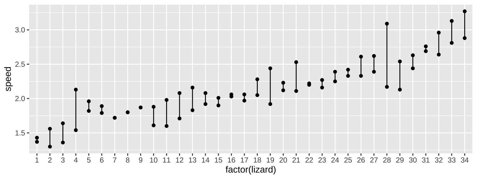
With random effects, we are interested in two sources of variation – that that is between individuals (or locations or whatever) and that that is within them. This sounds a lot like a fixed effects ANOVA, so that will be our starting place. Let’s look at this output, but ignore F and P as we don’t care about them for random effects.
lizard_runs <- lizard_runs %>% mutate( lizard = as.factor(lizard)) # we don't want R thinking lizard 3 is two more than lizard one
lizard_runs_lm <- lm(speed ~ lizard, data = lizard_runs)
anova(lizard_runs_lm)
Analysis of Variance Table
Response: speed
Df Sum Sq Mean Sq F value Pr(>F)
lizard 33 11.3219 0.34309 7.447 3.416e-08 ***
Residuals 34 1.5664 0.04607
---
Signif. codes: 0 '***' 0.001 '**' 0.01 '*' 0.05 '.' 0.1 ' ' 1We see that the mean square for groups (\(MS_{\text{group}}\))—the average squared difference between group means and the overall mean—is 0.34309. This value captures both the variability among lizards due to true differences in their average running speeds and variability due to chance sampling.
How much of this variability is due to true differences among lizards? To estimate this, we first recognize that the mean square error (\(MS_{\text{error}} = 0.04607\)) represents the variability within groups due to chance sampling. This is the amount of variability we expect to see in \(MS_{\text{group}}\) purely by chance.
To isolate the variability among lizards, we subtract \(MS_{\text{error}}\) from \(MS_{\text{group}}\). However, because each individual in a group contributes to the estimate of \(MS_{\text{group}}\), we divide the difference by the number of individuals per group (\(n_{\text{per group}}\)). This gives us the variance among lizards:
\[s_A^2 = \frac{MS_{\text{group}} - MS_{\text{error}}}{n_{\text{per group}}}\]
For this example:
\[s_A^2 = \frac{0.34309 - 0.04607}{2} = 0.1485\]
This means that if we could measure each lizard’s running speed an infinite number of times, the variance in their true average running speeds would be 0.1485. This value reflects the variability among lizards after accounting for random sampling error within groups.
A Random Effects Approach with the lme4 Package
For simple models, such as the example here, we can use an ANOVA table to estimate \(s_A^2\). However, as models become more complex and involve a mix of random and fixed effects, this approach becomes less feasible. To address this, we can use the lmer() function from the lme4 package to fit random and mixed-effects models (covered in the next section).
The syntax of lmer() is similar to lm(), but includes a language for specifying random effects. For instance, to estimate the variance (or standard deviations) in group means for a model where groups are random samples from a population, we use the following code:
library(lme4) # Install lme4 first if necessary
lizard_runs_rand <- lmer(speed ~ (1 | lizard), data = lizard_runs)
lizard_runs_rand
Linear mixed model fit by REML ['lmerModLmerTest']
Formula: speed ~ (1 | lizard)
Data: lizard_runs
REML criterion at convergence: 54.4173
Random effects:
Groups Name Std.Dev.
lizard (Intercept) 0.3854
Residual 0.2146
Number of obs: 68, groups: lizard, 34
Fixed Effects:
(Intercept)
2.139 logLik(lizard_runs_rand)'log Lik.' -27.20865 (df=3)Here’s what the output tells us:
“REML criterion at convergence”: This is two times the log-likelihood of the model:
\(2 \cdot \text{logLik}(\text{lizard_runs_rand}) =\) -54.4173045. Note compared to standard Maximum likelihood, REML incorporates uncertainty in our estimate of fixed effects – in this case the intercept.Std.Devforlizard: This is the square root of our estimate for the variance among lizards (\(s_A^2\)):
\(\sqrt{0.1485} = 0.385357\).Std.Devfor Residual: This represents the expected variability within groups, calculated as the square root of the mean square error:
\(\sqrt{0.04607} = 0.2146\).Fixed Effect (Intercept): This is our estimate for the overall mean:
summarize(lizard_runs, mean(speed)) =2.1391176.
Hypothesis Testing for Random Effects
To test the null hypothesis that the among-group variance is zero, we can perform a likelihood ratio test. This involves:
- Calculating two times the difference in log-likelihoods between the random-effects model and the null model.
- Comparing this value to the \(\chi^2\) distribution with one degree of freedom (since we estimate one parameter—the variance).
- Note: While REML is typically used for estimating random effects, maximum likelihood (ML) should be used for likelihood ratio tests, as REML log-likelihoods are not directly comparable between models with different fixed-effects structures.
# Output results (hidden from the document)
c(log_lik_rand = log_lik_rand, log_lik_null = log_lik_null, d = d, p = p)
log_lik_rand log_lik_null d p
-2.720865e+01 -4.195827e+01 2.949924e+01 5.593862e-08 Alternatively, we can use the ranova() function from the lmerTest package to perform this test:
ANOVA-like table for random-effects: Single term deletions

Model:
speed ~ (1 | lizard)
             npar  logLik    AIC    LRT Df Pr(>Chisq)
<none>          3 -27.209 60.417
(1 | lizard)    2 -41.958 87.917 29.499  1  5.594e-08 ***
---
Signif. codes:  0 '***' 0.001 '**' 0.01 '*' 0.05 '.' 0.1 ' ' 1
Repeatability
In a random-effects model, we estimate the variance among groups, \(s_A^2\). We may also want to assess what proportion of the total variance in the population is attributed to differences among groups. This measure, known as repeatability or the intraclass correlation coefficient (ICC), is calculated as:
\[\text{Repeatability} = \frac{s_A^2}{s_A^2 + MS_\text{error}}\]
A repeatability of zero means that measuring the same sample twice is no more consistent than taking two random samples, while a repeatability of one implies no variation within individuals (perfect consistency).
For our lizard running example:
\[\text{Repeatability} = \frac{0.1485}{0.1485 + 0.0461} = 0.763\]
This suggests that the measurements are highly repeatable.
Repeatability vs. \(R^2\)
Repeatability quantifies how similar measurements from the same group (e.g., a random lizard) are expected to be. It is meaningful only for random effects and is useful because it represents a parameter interpretable beyond the context of the specific model.
\(R^2\), in contrast, measures the proportion of variance “explained by the model” (\(SS_\text{groups}/SS_\text{total}\)) and is specific to the fixed-effects structure of a given experiment. Unlike repeatability, \(R^2\) cannot be generalized beyond the scope of the specific dataset.
In our example:
\[R^2 = \frac{11.3219}{11.3219 + 1.5664} = 0.8785\]
While both measures are related to variance, the difference is clear: \(R^2\) pertains to the model’s explanatory power, while repeatability pertains to the consistency of measurements within groups.
Shrinkage
From our understanding of “regression to the mean,” we know that extreme values are often overestimates. A valuable feature of the random-effects approach is that it leverages information across individuals, leading to “shrinkage.” In this context, shrinkage means that our estimates for individual groups are “pulled” toward the overall population mean.
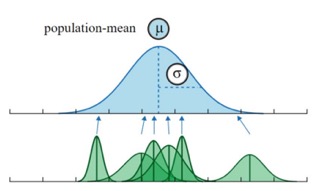
The extent of shrinkage depends on:
- The variability of the coefficients across clusters: Greater variability reduces shrinkage.
- The uncertainty associated with individual estimates: Higher uncertainty increases shrinkage.
Let’s explore this concept using our lizard running data.
First, we’ll grab predictions from our fixed-effects model:
Next, we’ll grab predictions from our random-effects model. Note here that we now require the broom.mixed package to tidy up output of mixed effects models witht he augment function:
Finally, we’ll combine these predictions and plot them. The “shrinkage” is evident as extreme estimates from the random-effects model are pulled toward the overall mean.
bind_rows(fixed_predicted_means, rand_predicted_means) %>%
  mutate(lizard = fct_reorder(lizard, .fitted, .fun = mean)) %>%
  ggplot(aes(x = lizard, y = .fitted, color = effect)) +
  geom_point() +
  geom_hline(yintercept = 2.139, linetype = "dashed") +
  labs(
    x = "Lizard",
    y = "Predicted Mean",
    color = "Model Type",
    title = "Shrinkage in Random-Effects Model Estimates"
  )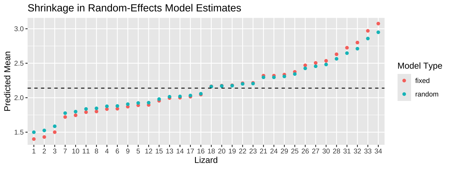
Here, the dashed horizontal line represents the overall mean, \(2.139\). Notice how the random-effects estimates are less extreme than those from the fixed-effects model, reflecting the shrinkage effect. This usually means that our predictions are more reliable reliable predictions, particularly when individual-level data is sparse or noisy. However, this depends on groups being truly random.
Assumptions of random effects models
Random effects models make our standard linear model assumptions and also assumes that groups (e.g. individuals, sites, etc.) are sampled at random and that group means are normally distributed. In the next section we see that by modeling random effects, we can model non-independence of observations.
Mixed-Effects Models
How do we test for some fixed effect, like if type of math instruction increases math scores,or if lizard sex is associated with sprint speed in the presence of this non-independence (like students in the same class learn from the same teacher, multiple measures of a lizard sprinting etc…)? In a mixed effect model, we model both fixed and random effects!!!! Mixed effect address non-independence within groups (by modeling the dependence structure of the data as a random effect) while simultaneously capturing systematic differences between groups (modeled as fixed effects).
For example, consider lizard sprint speeds:
- Measurements may be non-independent because multiple observations come from the same lizard (a random effect).
- Observations may also differ systematically because male and female lizards sprint at different speeds (a fixed effect).
In this case, we can model lizard as a random effect to account for variability among individuals and sex as a fixed effect to account for predictable differences between males and females.
When the focus of the analysis is not on the specific groups themselves (e.g., individual lizards), the variance among groups is referred to as a nuisance parameter. This random effect accounts for variation that isn’t of direct interest but must be considered to make accurate inferences.
When the grouping variable (lizard, or class, or whatever “cluster” we’re concerned with) is chosen at random, and that (beyond the fixed effects modelled) there is no relationship between individuals from different groups, we can model it as a random effect. If the observations from different groups are non-independent in ways that are not of direct interest (e.g., they have familial, temporal or spatial dependence), we need another approach.
Random Intercepts
With a “random intercept” each cluster gets its own intercept, which it drawn from some distribution. This on its own is much like the lizard example, above. If we assume a random intercept only, we assume that each cluster draws an intercept from some distribution, but that clusters have the same slope (save what is specified in the fixed effect).
Random Slopes
With a “random slope” each cluster gets its own slope, which it drawn from some distribution.
If we assume a random slope only, we assume that each cluster draws a slope from some distribution, but that cluster have the same intercepts (save what is specified in the fixed effect).
Random Slopes and Random Intercepts
We can, in theory model both random slopes and random intercepts. But sometimes these are hard to estimate together, so be careful.
Visualizing Random Intercepts and Random Slopes
I find it pretty hard to explain random slopes and intercepts in words, but that pictures really help!
Read and scroll through the example below, as it is the best description I’ve come across (for some reason, the embedded app has been finicky, so if it doesn’t show up go directly to the website here.
Mixed model: Random intercept example
Selenium, is a bi-product of burning coal. Could Selenium bioaccumulate in fish, suchb that fish from lakes with more selenium have more selenium in them?
Let us look at data (download here) from 98 fish from nine lakes, with 1 to 34 fish per lake.
Ignoring nonindependence is inappropriate
What if we just ignored lake and assumed each fish was independent???
selenium     <- read_csv("https://drive.google.com/uc?export=download&id=1UAkdZYLJPWRuFrq9Dc4StxfHCGW_43Ye")
selenium_lm1 <- lm(Log_fish_Se ~  Log_Water_Se, data = selenium)

summary(selenium_lm1)
Call:
lm(formula = Log_fish_Se ~ Log_Water_Se, data = selenium)

Residuals:
    Min      1Q  Median      3Q     Max
-0.7569 -0.3108 -0.1789  0.4301  0.8180

Coefficients:
             Estimate Std. Error t value Pr(>|t|)
(Intercept)   1.16351    0.06387  18.216  < 2e-16 ***
Log_Water_Se  0.26483    0.05858   4.521 2.08e-05 ***
---
Signif. codes:  0 '***' 0.001 '**' 0.01 '*' 0.05 '.' 0.1 ' ' 1

Residual standard error: 0.4305 on 81 degrees of freedom
Multiple R-squared:  0.2015,    Adjusted R-squared:  0.1916
F-statistic: 20.44 on 1 and 81 DF, p-value: 2.081e-05anova(selenium_lm1)Analysis of Variance Table
Response: Log_fish_Se
Df Sum Sq Mean Sq F value Pr(>F)
Log_Water_Se 1 3.787 3.7870 20.436 2.081e-05 ***
Residuals 81 15.010 0.1853
---
Signif. codes: 0 '***' 0.001 '**' 0.01 '*' 0.05 '.' 0.1 ' ' 1ggplot(selenium, aes(x = Log_Water_Se, y = Log_fish_Se, label = Lake)) +
geom_point(aes(color = Lake), alpha = .5, size = 3) +
geom_smooth(method = "lm")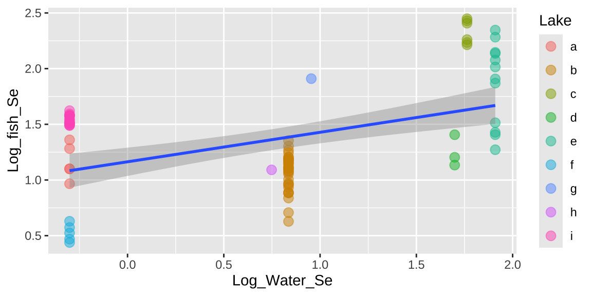
That would be a big mistake – as each fish is not independent. There could be something else about the lake associated with levels of Selenium in fish that is not in our model. This seems likely, as we see below, that residuals differ substantially by lake.
bind_cols( selenium ,
           augment(selenium_lm1)  %>%    dplyr::select(.resid))%>%
  ggplot(aes(x = Lake, y = .resid, color = Lake)) +
  geom_jitter(width = .2, size = 3, alpha =.6, show.legend = FALSE)+
  geom_hline(yintercept = 0, color = "red")+
  stat_summary(data = . %>% group_by(Lake) %>% mutate(n = n()) %>% dplyr::filter(n>1), color = "black")
So why is this so bad? It’s because we keep pretending each fish is independent when it is not. So, our certainty is WAY bigger than it deserves to be. This means that our p-value is WAY smaller than it deserves to be.
We can’t model lake as a fixed effect
And even if we could it would be wrong.
Putting lake into our model as a fixed effect would essentially take the average of Fish Selenium content for each lake. Since each lake has only one Selenium content, we then have nothing to model (as sen by the NA for our estimate of the effect of lake selenium content on fish selenium concentration).
lm(Log_fish_Se ~ Lake + Log_Water_Se, data = selenium) | parameter | estimate |
|---|---|
| (Intercept) | 1.162 |
| Lakeb | -0.089 |
| Lakec | 1.171 |
| Laked | 0.086 |
| Lakee | 0.705 |
| Lakef | -0.635 |
| Lakeg | 0.748 |
| Lakeh | -0.071 |
| Lakei | 0.379 |
| Log_Water_Se | NA |
But even when this is not the case, this is not the appropriate modelling strategy.
Taking averages is a less wrong thing
What if we just took the average selenium content over all fish for every lake, and then did our stats?
selenium_avg <- selenium %>%
  group_by(Lake, Log_Water_Se) %>%
  summarise(mean_log_fish_Se = mean(Log_fish_Se), n = n())

selenium_lm2 <- lm(mean_log_fish_Se ~  Log_Water_Se, data = selenium_avg)
summary(selenium_lm2)
Call:
lm(formula = mean_log_fish_Se ~ Log_Water_Se, data = selenium_avg)

Residuals:
     Min       1Q   Median       3Q      Max
-0.50657 -0.36536  0.03456  0.42871  0.55425

Coefficients:
             Estimate Std. Error t value Pr(>|t|)
(Intercept)    1.1307     0.2094   5.399  0.00101 **
Log_Water_Se   0.3673     0.1807   2.032  0.08161 .
---
Signif. codes:  0 '***' 0.001 '**' 0.01 '*' 0.05 '.' 0.1 ' ' 1

Residual standard error: 0.4653 on 7 degrees of freedom
Multiple R-squared:  0.3711,    Adjusted R-squared:  0.2813
F-statistic: 4.131 on 1 and 7 DF, p-value: 0.08161anova(selenium_lm2)Analysis of Variance Table
Response: mean_log_fish_Se
Df Sum Sq Mean Sq F value Pr(>F)
Log_Water_Se 1 0.89428 0.89428 4.131 0.08161 .
Residuals 7 1.51536 0.21648
---
Signif. codes: 0 '***' 0.001 '**' 0.01 '*' 0.05 '.' 0.1 ' ' 1ggplot(selenium_avg, aes(x = Log_Water_Se, y = mean_log_fish_Se, label = Lake)) +
geom_point(aes(size = n)) +
geom_text_repel(aes(color = Lake), show.legend = FALSE) +
geom_smooth(method = "lm",se = FALSE)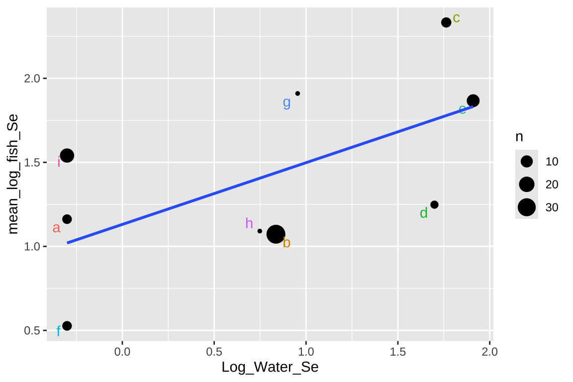
This approach isn’t too bad, but there are some shortcomings –
- It takes all means as equally informative, even though some come from large and others from large samples.
- It ignores variability within each lake,
- It surrenders so much of our hard-won data.
Accounting for Lake as a Random Effect is our best option
Rather, we can model Lake as a random effect – this allows us to model the non-independence of observations within a Lake, while using all of the data.
Linear mixed model fit by REML. t-tests use Satterthwaite's method [
lmerModLmerTest]
Formula: Log_fish_Se ~ (1 | Lake) + Log_Water_Se
   Data: selenium

REML criterion at convergence: -8.8

Scaled residuals:
     Min       1Q   Median       3Q      Max
-3.15542 -0.37400  0.04239  0.54953  2.54730

Random effects:
 Groups   Name        Variance Std.Dev.
 Lake     (Intercept) 0.20747  0.4555
 Residual             0.03548  0.1884
Number of obs: 83, groups:  Lake, 9

Fixed effects:
             Estimate Std. Error     df t value Pr(>|t|)
(Intercept)    1.1322     0.2089 6.8420   5.419  0.00107 **
Log_Water_Se   0.3659     0.1794 6.7266   2.039  0.08249 .
---
Signif. codes:  0 '***' 0.001 '**' 0.01 '*' 0.05 '.' 0.1 ' ' 1

Correlation of Fixed Effects:
            (Intr)
Log_Water_S -0.666
Thus we fail to reject the null, and conclude that there is not sufficient evidence to support the idea that more selenium in lakes is associated with more selenium in fish.
Extracting estimates and uncertainty
Although we do have model estimates, degrees of freedom, and standard deviations above, if can still be hard to consider and communicate uncertainty. The ggpredict() function in the ggeffects package can help!
library(ggeffects)
gg_color_hue <- function(n) {hues = seq(15, 375, length = n + 1); hcl(h = hues, l = 65, c = 100)[1:n]}

selenium_predictions <- ggpredict(selenium_lme, terms = "Log_Water_Se")
selenium_predictions
# Predicted values of Log_fish_Se
Log_Water_Se | Predicted | 95% CI
-------------------------------------
-0.30 | 1.02 | 0.53, 1.52
0.75 | 1.41 | 1.10, 1.72
0.84 | 1.44 | 1.13, 1.75
0.95 | 1.48 | 1.16, 1.80
1.70 | 1.75 | 1.30, 2.21
1.76 | 1.78 | 1.31, 2.25
1.91 | 1.83 | 1.32, 2.34
Adjusted for:
* Lake = 0 (population-level)plot(selenium_predictions)+
geom_jitter(data = selenium, aes(x = Log_Water_Se , y= Log_fish_Se, color = Lake), alpha = .4, size = 3,height = 0, width = .02)+
scale_color_manual(values = gg_color_hue(9))+
labs(color = "Lake")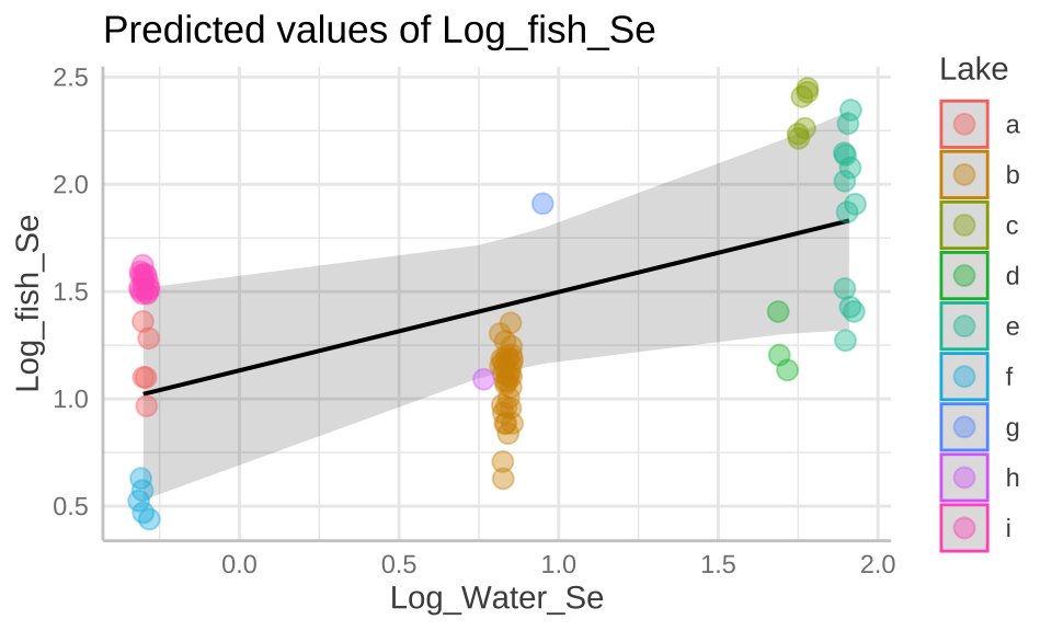
Evaluating assumptions
We can now see that by modeling Lake as a random effect, the residuals are now independent.
bind_cols( selenium ,
           broom.mixed::augment(selenium_lme)  %>%    dplyr::select(.resid))%>%
  ggplot(aes(x = Lake, y = .resid, color = Lake)) +
  geom_jitter(width = .2, size = 3, alpha =.6, show.legend = FALSE)+
  geom_hline(yintercept = 0, color = "red")+
  stat_summary(data = . %>% group_by(Lake) %>% mutate(n = n()) %>% dplyr::filter(n>1),color = "black")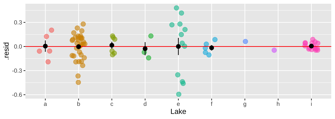
Major assumptions of linear mixed effect models are
- Data are collected without bias
- Clusters are random
- Data can be modelled as a linear function of predictors
- Variance of the residuals is independent of predicted values,
- Residuals are normally distributed,
Let’s look into the last two for these data. Because autoplot can’t handle random effects output, let’s make out own diagnostic plots, again we use the augment() function from the broom.mixed package.
library(broom.mixed)
selenium_qq <- broom.mixed::augment(selenium_lme) %>%
  ggplot(aes(sample = .resid))+
  geom_qq()+
  geom_qq_line()

selenium_std_resid  <- broom.mixed::augment(selenium_lme) %>%
  mutate(sqrt_abs_std_resid = sqrt(abs(.resid / sd(.resid)) )) %>%
  ggplot(aes(x = .fitted, y = sqrt_abs_std_resid)) +
  geom_point()

plot_grid(selenium_qq, selenium_std_resid, ncol = 2)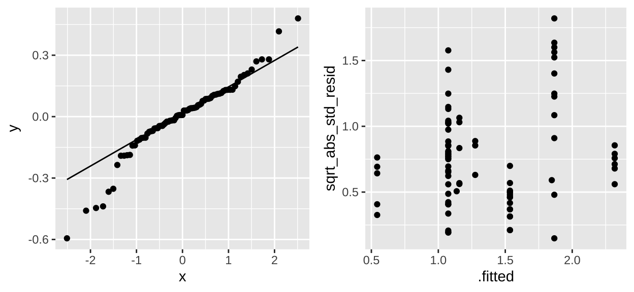
These don’t look great tbh. We would need to think harder if we were doing a legitimate analysis.
Example II: Loblolly Pine Growth
Let’s try to model the growth rate of loblolly pines!
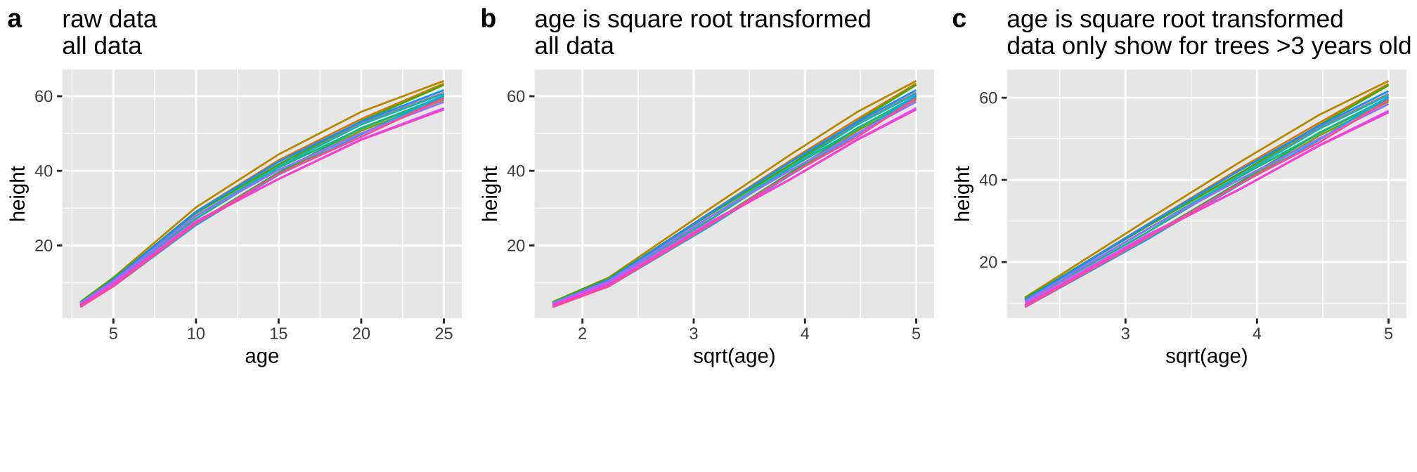
First I looked at the data (a), and thought a square root transform would be a better linear model (b), especially if I began my model after three years of growth (c).
Random Slopes
loblolly_rand_slope <- lmer(height ~ sqrt(age)+ (0+age|Seed),
                            data = filter(Loblolly, age>3))
summary(loblolly_rand_slope)
Linear mixed model fit by REML. t-tests use Satterthwaite's method [
lmerModLmerTest]
Formula: height ~ sqrt(age) + (0 + age | Seed)
Data: filter(Loblolly, age > 3)
REML criterion at convergence: 203.5
Scaled residuals:
Min 1Q Median 3Q Max
-1.95946 -0.58072 -0.02036 0.66442 1.69493
Random effects:
Groups Name Variance Std.Dev.
Seed age 0.01104 0.1050
Residual 0.54136 0.7358
Number of obs: 70, groups: Seed, 14
Fixed effects:
Estimate Std. Error df t value Pr(>|t|)
(Intercept) -30.4798 0.4796 45.5371 -63.55 <2e-16 ***
sqrt(age) 18.3506 0.2161 18.5472 84.92 <2e-16 ***
---
Signif. codes: 0 '***' 0.001 '**' 0.01 '*' 0.05 '.' 0.1 ' ' 1
Correlation of Fixed Effects:
(Intr)
sqrt(age) -0.916broom.mixed::augment(loblolly_rand_slope) %>% mutate(Seed = as.character(Seed)) %>%
ggplot(aes(x = `sqrt(age)`, y = .fitted, color = Seed)) +
geom_line() + theme(legend.position = "none")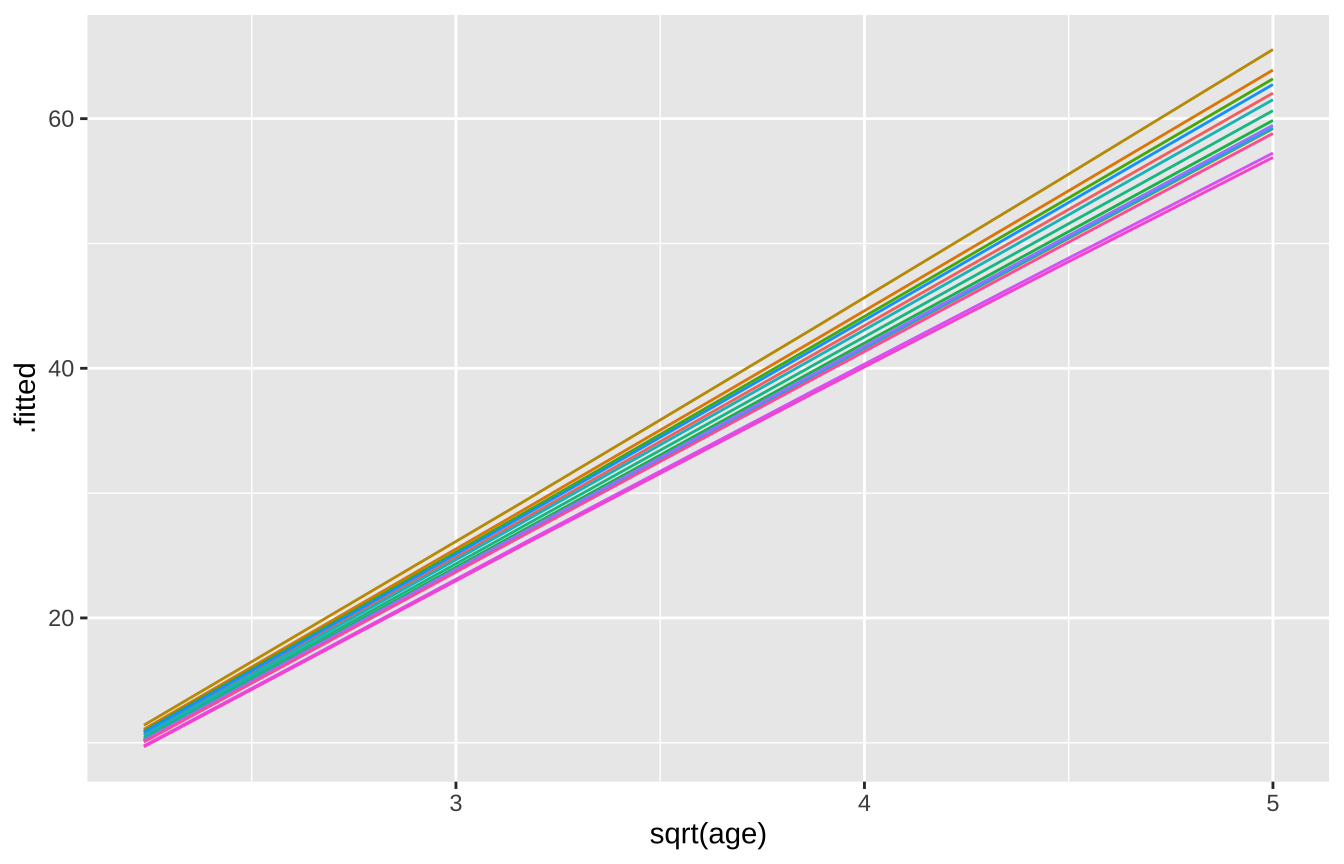
Random Intercepts
loblolly_rand_intercept <- lmer(height ~ sqrt(age) + (1|Seed),
                                data = filter(Loblolly, age>3))
summary(loblolly_rand_intercept)
Linear mixed model fit by REML. t-tests use Satterthwaite's method [
lmerModLmerTest]
Formula: height ~ sqrt(age) + (1 | Seed)
Data: filter(Loblolly, age > 3)
REML criterion at convergence: 224.2
Scaled residuals:
Min 1Q Median 3Q Max
-2.33172 -0.60269 -0.05526 0.72322 1.84426
Random effects:
Groups Name Variance Std.Dev.
Seed (Intercept) 2.6310 1.622
Residual 0.8118 0.901
Number of obs: 70, groups: Seed, 14
Fixed effects:
Estimate Std. Error df t value Pr(>|t|)
(Intercept) -30.2214 0.6096 38.3445 -49.58 <2e-16 ***
sqrt(age) 18.1960 0.1106 55.0000 164.45 <2e-16 ***
---
Signif. codes: 0 '***' 0.001 '**' 0.01 '*' 0.05 '.' 0.1 ' ' 1
Correlation of Fixed Effects:
(Intr)
sqrt(age) -0.680broom.mixed::augment(loblolly_rand_intercept) %>% mutate(Seed = as.character(Seed)) %>%
ggplot(aes(x = `sqrt(age)`, y = .fitted, color = Seed)) +
geom_line() + theme(legend.position = "none")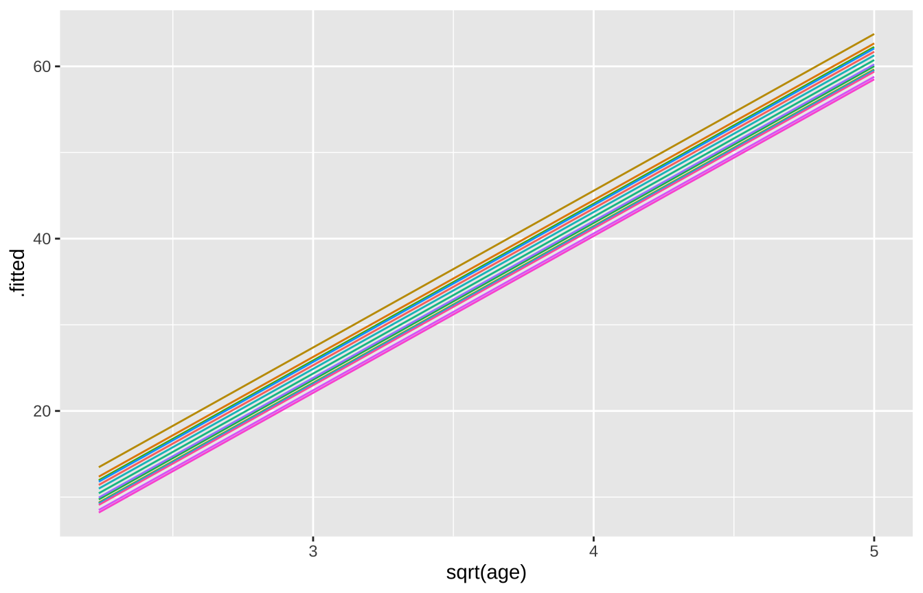
Conclusion
After accounting for the effect of seed by modelling it as a random effect, we find that trees reliably increase in height with age. We see a similar increase whether we model seed as a random slope or intercept.
Additional related topics
Sadly our term is coming to an end, as we are just beginning to explore these more complex, flexible, and realistic models. In this brief section, I will show you a few fun directions for more complex models. If you are interested in these problems, I highly recommend John Fieberg’s fantastic course – FW8051 Statistics for Ecologists. Check out his book here.
Generalized Least Squares
We can still run into issues of heteroscedasticity and hierarchical model structure with non-random groups. For such cases, we can use generalized least squares. In R, we can do this with the gls() function in the nlme package.
More complex covariance structures
We have considered a simple random effect where individuals are in one group or another. Sometimes the world i more complicated – for example if we have random families, individuals within the family are not equally related. We therefore want to specify more realistic covariances of residuals. In R, we can do this with the lme() function in the nlme package.
Generalized Linear Mixed Effect Models
We previously saw that we could generalize a linear model to nonlinear distributions. We can do the same for mixed effects models. We can do this with the glmer() function in lme4. These can be a bit tricky, so proceed with caution.
Quiz
Figure 1: Quiz on random and mixed effect models here